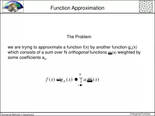
Function Approximation
Function Approximation. Function approximation (Chapters 13 & 14) -- method of least squares -- minimize the residuals -- given data of points have noises -- the purpose is to find the trend represented by data. Function interpolation (Chapters 15 & 16)

Function Approximation
E N D
Presentation Transcript
Function Approximation • Function approximation (Chapters 13 & 14) -- method of least squares -- minimize the residuals -- given data of points have noises -- the purpose is to find the trend represented by data. • Function interpolation (Chapters 15 & 16) -- approximating function match the given data exactly -- given data of points are precise -- the purpose is to find data between these points
Chapter 13 Curve Fitting: Fitting a Straight Line
Least Square Regression • Curve Fitting • Statistics Review • Linear Least Square Regression • Linearization of Nonlinear Relationships • MATLAB Functions
Wind Tunnel Experiment Curve Fitting Measure air resistance as a function of velocity
Regression and Interpolation Curve fitting (a) Least-squares regression (b) Linear interpolation (c) Curvilinear interpolation
Least-squares fit of a straight line v, m/s F, N
Simple Statistics Measurement of the coefficient of thermal expansion of structural steel [106 in/(inF)] Mean, standard deviation, variance, etc.
Statistics Review • Arithmetic mean • Standard deviationabout the mean • Variance (spread) • Coefficient of variation (c.v.)
1 6.485 0.007173 42.055 2 6.554 0.000246 42.955 3 6.775 0.042150 45.901 4 6.495 0.005579 42.185 5 6.325 0.059875 40.006 6 6.667 0.009468 44.449 7 6.552 0.000313 42.929 8 6.399 0.029137 40.947 9 6.543 0.000713 42.811 10 6.621 0.002632 43.838 11 6.478 0.008408 41.964 12 6.655 0.007277 44.289 13 6.555 0.000216 42.968 14 6.625 0.003059 43.891 15 6.435 0.018143 41.409 16 6.564 0.000032 43.086 17 6.396 0.030170 40.909 18 6.721 0.022893 45.172 19 6.662 0.008520 44.382 20 6.733 0.026669 45.333 21 6.624 0.002949 43.877 22 6.659 0.007975 44.342 23 6.542 0.000767 42.798 24 6.703 0.017770 44.930 25 6.403 0.027787 40.998 26 6.451 0.014088 41.615 27 6.445 0.015549 41.538 28 6.621 0.002632 43.838 29 6.499 0.004998 42.237 30 6.598 0.000801 43.534 31 6.627 0.003284 43.917 32 6.633 0.004008 43.997 33 6.592 0.000498 43.454 34 6.670 0.010061 44.489 35 6.667 0.009468 44.449 36 6.535 0.001204 42.706 236.509 0.406514 1554.198
Coefficient of Thermal Expansion Mean Sum of the square of residuals Standard deviation Variance Coefficient of variation
Histogram Normal Distribution • A histogram used to depict the distribution of data • For large data set, the histogram often approaches the normal distribution (use data in Table 12.2)
Linear Regression Fitting a straight line to observations Small residual errors Large residual errors
Linear Regression • Equation for straight line • Difference between observation and line • ei is the residual or error
Least Squares Approximation • Minimizing Residuals (Errors) • minimum average error (cancellation) • minimum absolute error • minimax error (minimizing the maximum error) • least squares (linear, quadratic, ….)
Minimize Sum of Errors Minimize Sum of Absolute Errors Minimize the Maximum Error
Linear Least Squares • Minimize total square-error • Straight line approximation • Not likely to pass all points if n > 2
Linear Least Squares • Total square-error function: sum of the squares of the residuals • Minimizing square-error Sr(a0 ,a1) Solve for (a0 ,a1)
Linear Least Squares • Minimize • Normal equation y = a0 + a1x
Advantage of Least Squares • Positive differences do not cancel negative differences • Differentiation is straightforward • weighted differences • Small differences become smaller and large differences are magnified
Linear Least Squares • Use sum( ) in MATLAB
Correlation Coefficient • Sum of squares of the residuals with respect to the mean • Sum of squares of the residuals with respect to the regression line • Coefficient of determination • Correlation coefficient
Correlation Coefficient • Alternative formulation of correlation coefficient • More convenient for computer implementation
Standard Error of the Estimate • If the data spread about the line is normal • “Standard deviation” for the regression line Standard error of the estimate No error if n = 2 (a0and a1)
Linear regression reduce the spread of data Spread of data around the mean Normal distributions Spread of data around the best-fit line
Standard Deviation for Regression Line Sy/x Sy Sy : Spread around the mean Sy/x : Spread around the regression line
Example: Linear Regression Standard deviation about the mean Standard error of the estimate Correlation coefficient
» x=1:7 x = 1 2 3 4 5 6 7 » y=[0.5 2.5 2.0 4.0 3.5 6.0 5.5] y = 0.5000 2.5000 2.0000 4.0000 3.5000 6.0000 5.5000 » s=linear_LS(x,y) a0 = 0.0714 a1 = 0.8393 x y (a0+a1*x) (y-a0-a1*x) 1.0000 0.5000 0.9107 -0.4107 2.0000 2.5000 1.7500 0.7500 3.0000 2.0000 2.5893 -0.5893 4.0000 4.0000 3.4286 0.5714 5.0000 3.5000 4.2679 -0.7679 6.0000 6.0000 5.1071 0.8929 7.0000 5.5000 5.9464 -0.4464 err = 2.9911 Syx = 0.7734 r = 0.9318 s = 0.0714 0.8393 Sum of squares of residuals Sr Standard error of the estimate Correlation coefficient y =0.0714 + 0.8393 x
» x=0:1:7; y=[0.5 2.5 2 4 3.5 6.0 5.5]; Linear regression y = 0.0714+0.8393x Error :Sr = 2.9911 correlation coefficient : r = 0.9318
function [x,y] = example1 x = [ 1 2 3 4 5 6 7 8 9 10]; y = [2.9 0.5 -0.2 -3.8 -5.4 -4.3 -7.8 -13.8 -10.4 -13.9]; » [x,y]=example1; » s=Linear_LS(x,y) a0 = 4.5933 a1 = -1.8570 x y (a0+a1*x) (y-a0-a1*x) 1.0000 2.9000 2.7364 0.1636 2.0000 0.5000 0.8794 -0.3794 3.0000 -0.2000 -0.9776 0.7776 4.0000 -3.8000 -2.8345 -0.9655 5.0000 -5.4000 -4.6915 -0.7085 6.0000 -4.3000 -6.5485 2.2485 7.0000 -7.8000 -8.4055 0.6055 8.0000 -13.8000 -10.2624 -3.5376 9.0000 -10.4000 -12.1194 1.7194 10.0000 -13.9000 -13.9764 0.0764 err = 23.1082 Syx = 1.6996 r = 0.9617 s = 4.5933 -1.8570 r = 0.9617 y = 4.5933 1.8570 x
Linear Least Square y = 4.5933 1.8570 x Error Sr = 23.1082 Correlation Coefficient r = 0.9617
» [x,y]=example2 x = Columns 1 through 7 -2.5000 3.0000 1.7000 -4.9000 0.6000 -0.5000 4.0000 Columns 8 through 10 -2.2000 -4.3000 -0.2000 y = Columns 1 through 7 -20.1000 -21.8000 -6.0000 -65.4000 0.2000 0.6000 -41.3000 Columns 8 through 10 -15.4000 -56.1000 0.5000 » s=Linear_LS(x,y) a0 = -20.5717 a1 = 3.6005 x y (a0+a1*x) (y-a0-a1*x) -2.5000 -20.1000 -29.5730 9.4730 3.0000 -21.8000 -9.7702 -12.0298 1.7000 -6.0000 -14.4509 8.4509 -4.9000 -65.4000 -38.2142 -27.1858 0.6000 0.2000 -18.4114 18.6114 -0.5000 0.6000 -22.3720 22.9720 4.0000 -41.3000 -6.1697 -35.1303 -2.2000 -15.4000 -28.4929 13.0929 -4.3000 -56.1000 -36.0539 -20.0461 -0.2000 0.5000 -21.2918 21.7918 err = 4.2013e+003 Syx = 22.9165 r = 0.4434 s = -20.5717 3.6005 Data in arbitrary order Large errors !! Correlation coefficient r = 0.4434 Linear Least Square: y = 20.5717 + 3.6005x
Linear regression y = 20.5717 +3.6005x Error Sr = 4201.3 Correlation r = 0.4434 !!
Untransformed power equationx vs. ytransformed datalog x vs. log y
Linearization of Nonlinear Relationships • Exponential equation • Power equation log : Base-10
Linearization of Nonlinear Relationships • Saturation-growth-rate equation • Rational function
Example 12.4: Power Equation Transformed Data log xi vs. log yi y = 2 x 2 Power equation fit along with the data x vs. y
>> x=[10 20 30 40 50 60 70 80]; >> y = [25 70 380 550 610 1220 830 1450]; >> [a, r2] = linregr(x,y) a = 19.4702 -234.2857 r2 = 0.8805 y = 19.4702x 234.2857 12-12
>> x=[10 20 30 40 50 60 70 80]; >> y = [25 70 380 550 610 1220 830 1450]; >> linregr(log10(x),log10(y)) r2 = 0.9481 ans = 1.9842 -0.5620 log y = 1.9842 log x – 0.5620 y = (10–0.5620)x1.9842 =0.2742x1.9842 log x vs. log y 12-13
MATLAB Functions • Least-square fit of nth-order polynomial p = polyfit(x,y,n) • Evaluate the value of polynomial using y = polyval(p,x)
CVEN 302-501Homework No. 9 • Chapter 13 • Prob. 13.1 (20)& 13.2(20) (Hand Calculations) • Prob. 13.5 (30) & 13.7(30) (Hand Calculation and MATLAB program) • You may use spread sheets for your hand computation • Due Oct/22, 2008 Wednesday at the beginning of the period