Download
1 / 71
710 likes | 824 Vues
Delve into constraints and patterns of abundance, wealth distribution theories, and feasible sets in ecology and economics through combinatorial analysis.

E N D
Combinatorial insight into a common pattern: uneven distributions of wealth and abundance Ken Locey
Constraint-based Ecology Physiological constraints Body size and metabolism
Constraint-based Ecology Physical constraints Body size and prey capture Evolutionary constraints Adaptation to new thermal regimes
Constraint-based Ecology Numerical constraints Total abundance (N) Species richness (S) S ≤ N
Rank-abundance curve (RAC) Species abundance distribution (SAD) Frequency distribution frequency Abundance Rank in abundance Abundance class
The ubiquitous hollow-curve frequency 0 1 2 3 4 5 6 7 Abundance class
Poverty in Rural America, 2008 54 – 25.1 25 – 20.1 12 – 10.1 10 – 3.1 20 – 14.1 14 – 12.1 Percent in Poverty
“Supreme importance attaches to one economic problem, the distribution of wealth. Is there a natural law according to which the income of society is divided?” John Bates Clark (1899) Wealth: sources of human welfare which are material, transferable, & limited in quantity.
Distributions used to predict variation in wealth, size, & abundance • Pareto (80-20 rule) • Log-normal • Log-series • Geometric series • Dirichlet • Negative binomial • Zipf • Zipf-Mandelbrot
Rank-abundance curve (RAC) Predicting, modeling, & explaining the Species abundance distribution (SAD) Frequency distribution frequency Abundance Rank in abundance Abundance class
Predicting, modeling, & explaining the Species abundance distribution (SAD) 104 Observed Resource partitioning Demographic stochasticity 103 Abundance 102 101 100 Rank in abundance
104 N = 1,700 S = 17 103 Abundance 102 101 100 Rank in abundance
How many forms of the SAD for a given N and S? 104 103 Abundance 102 101 100 Rank in abundance
Integer Partitioning Integer partition: A positive integer expressedas the sum of unordered positive integers e.g. 6 = 3+2+1 = 1+2+3 = 2+1+3 Written in non-increasing (lexical) order e.g. 3+2+1
Rank-abundance curves are integer partitions Rank-abundance curve Integer partition N = total abundance S = species richness Sunlabeled abundances that sum to N N = positive integer S = number of parts Sunordered +integers that sum to N =
Random integer partitions Nijenhuis and Wilf (1978) Combinatorial Algorithms for Computer and Calculators. Academic Press, New York. Goal: Random partitions for N = 5, S = 3: 3+1+1 2+2+1
SAD feasible sets aredominated by hollow curves Frequency log2(abundance)
The SAD feasible set N=1000, S=40 ln(abundance) Rank in abundance
Question Can we explain variation in abundance based on how N and S constrain observable variation?
Sampling the SAD feasible Set Sample size = 300 Sample size = 500 Sample size = 700 Density Density Density Evenness Evenness Evenness
The center ofthe feasible set N=1000, S=40 ln(abundance) Rank in abundance
R2 = 1.0 102 101 100 Observed abundance R2 per site 100 101 102 Abundance at the center of the feasible set
Breeding Bird Survey (1,583 sites) R2 = 0.93 102 101 100 Observed abundance R2 per site 100 101 102 Abundance at the center of the feasible set
Observed abundance Abundance at center of the feasible set
Observed abundance Abundance at center of the feasible set
Public code and data repository https://github.com/weecology/feasiblesets
General Conclusions We shouldaccount for how generalvariables constrain ecological patterns ...beforeattributing the form of a pattern to a process
General Conclusions Observable variation in the SAD explains the ubiquitous hollow-curve
General Conclusions Extending the feasible set approach: • Spatial abundance distribution • Species area relationship • Distributions of wealth and abundance
0.93 0.88 0.91 0.91 Observed home runs 0.94 0.93 Center of the feasible set http://mlb.mlb.com
“Is there a natural law according to which the income of society is divided?” John Bates Clark (1899) The uneven nature of nature: Most of the possible shapes of a distribution of wealth are hollow-curves
General Conclusions Combinatorics is one only way to examine feasible sets Other (more common) ways: Mathematical optimization Linear programming
Efficient algorithms for sampling integerpartition feasible sets
Combinatorial Explosion Probability of generating a random partition of 1000 having 10 parts:< 10-17
Task: Generate random partitions of N=9 having S=4 parts 4+3+2
3+3+2+1 4+3+2