
Correlations
E N D
Presentation Transcript
Correlations Inferential Statistics
Overview • Correlation coefficients • Scatterplots • Calculating Pearson’s r • Interpreting correlation coefficients • Calculating & interpreting coefficient of determination • Determining statistical significance • Calculating Spearman’s correlation coefficient
Correlation • Reflects the degree of relation between variables • Calculation of correlation coefficient • Direction • + (positive) or – (negative) • Strength (i.e., magnitude) • Further away from zero, the stronger the relation • Form of the relationship
Check yourself • Indicate whether the following statements suggest a positive or negative relationship: • High school students with lower IQs have lower GPAs • More densely populated areas have higher crime rates • Heavier automobiles yield poorer gas mileage • More anxious people willingly spend more time performing a simple repetitive task
Correlation & Scatterplots r= .91 • Benefits of scatterplot • Form of relation • Any possible outliers? • Rough guess of r
Correlation & Scatterplots # of times arrested
Pearson’s r • Formula • SP = Sum of products (of deviations) • SSx = Sum of Squares of X • SSy = Sum of Squares of Y
Pearson’s r • Calculating SP • Definitional formula • Computational formula • Find X & Y deviations for each individual • Find product of deviations for each individual • Sum the products
Example #1Calculating SP – Definitional Formula Step 2: Multiply the deviations from the mean Step 3: Sum the products SX = 12 SY = 16 MX = SX/n = 12/4 = 3 MY = SY/n = 16/4 = 4 Step 1: Find deviations for X and Y separately
Example #1Calculating SP – Computational Formula SX = 12 SY = 16 MX = SX/n = 12/4 = 3 MY = SY/n = 16/4 = 4
Calculating Pearson’s r • Calculate SP • Calculate SS for X • Calculate SS for Y • Plug numbers into formula
Calculating Pearson’s r • Calculate SP • Calculate SS for X • Calculate SS for Y • Plug numbers into formula
Example #1 - AnswersCalculating Pearson’s r SX = 12 SY = 16 MX = SX/n = 12/4 = 3 MY = SY/n = 16/4 = 4
Pearson’s r • r = covariability of X and Y variability of X and Y separately
Using Pearson’s r • Prediction • Validity • Reliability
Verbal Descriptions • 1) r = -.84 between total mileage & auto resale value • 2) r = -.35 between the number of days absent from school & performance on a math test • 3) r = -.05 between height & IQ • 4) r = .03 between anxiety level & college GPA • 5) r = .56 between age of schoolchildren & reading comprehension level
Interpreting correlations • Describe a relationship between 2 vars • Correlation does not equal causation • Directionality Problem • Third-variable Problem • Restricted range • Obscures relationship
Interpreting correlations • Outliers • Can have BIG impact on correlation coefficient
Interpreting correlations • Strength & Prediction • Coefficient of determination r2 • Proportion of variability in one variable that can be determined from the relationship w/ the other variable • r = .60, then r2 = .36 or 36% • 36% of the total variability in X is consistently associated with variability in Y • “predicted” and “accounted for” variability
Mini-Review • Correlations • Calculation of Pearson’s r • Sum of product deviations • Using Pearson’s r • Verbal descriptions • Interpretation of Pearson’s r
Example #2Practice – Calculate Pearson’s r • Calculate SP • Calculate SS for X • Calculate SS for Y • Plug numbers into formula
Example #2 SP = S(X-MX)(Y-MY) SSY SX = 10 SY = 35 MX = SX/n = 10/5 = 2 MY = SY/n = 35/5 = 7 SSX
Hypothesis Testing • Making inferences based on sample information • Is it a statistically significant relationship? Or simply chance?
= 3 With n=5, there can be only 4 df Conceptually - Degrees of freedom • Knowing M (the mean) restricts variability in sample • 1 score will be dependent on others • n = 5, SX = 20 • If we know first 3 scores • If we know first 4 scores Score X1 = 6 X2 = 4 X3 = 2 X4 X5 Σx= 20 = 5
Correlations – Degrees of freedom • There are no degrees of freedom when our sample size is 2. When there are only two points on a scatterplot, they will fit perfectly on a straight line. • Thus, for correlations df= n – 2
Using table to determine significance • Find degrees of freedom • Correlations: df= n – 2 • Use level of significance (e.g., a = .05) for two-tailed test to find column in Table • Determine critical value • Value calculated r must equal or exceed to be significant • Compare calculated r w/ critical value • If calculated r less than critical value = not significant • APA • The correlation between hours watching television and amount of aggression is not significant, r (3) = -.80, p > .05. Think about sample size
Spearman correlation • Used when: • Ordinal data • If 1 variable is on ratio scale, then change scores for that variable into ranks Difference between pair of ranks
Example #4: Spearman Correlation • Two movie raters each watched the same six movies. Is there are relationship between the raters’ rankings?
Pearson r (from SPSS) Spearman rs (from SPSS)
Example #5: Pearson’s r Participant Motivation (X)Depression (Y) 1 3 8 2 6 4 3 9 2 4 2 2 • Sketch a scatterplot. • Calculate the correlation coefficient. • Determine if it is statistically significant at the .05 level for a 2-tailed test. • Write an APA format conclusion.