Assessing Normality in Data Using the 68-95-99.7 Rule and Normal Probability Plots
This guide provides a comprehensive approach to assessing the normality of data, utilizing the 68-95-99.7 rule. It outlines the steps for plotting data to check for shape, including determining the percentage of data within specific standard deviations. Learn to create Normal Probability Plots by converting data values to z-scores and analyzing their linearity. The visual representation will help identify any skewness. We apply these techniques to a practical example involving the capacities of side-by-side refrigerators, enhancing your understanding of these statistical concepts.

Assessing Normality in Data Using the 68-95-99.7 Rule and Normal Probability Plots
E N D
Presentation Transcript
Assessing Normality When is the data Normal enough?
Use the 68-95-99.7 Rule • Plot the data and check for the shape to be……. • Determine if ____ % of the data is within 1 standard deviation • Determine if 95% of the data is within ___ standard deviations • Determine if ____ % of the data is within ____ standard deviations
Normal Probability Plot • X-axis is the data scale • Y-axis is the z-score scale • All data is converted to its z-score and plotted as (data, z-score) • Data should appear linear if it is Normal
Shape from Normal Probability Plot • Symmetric = Linear • Skewed Right = few large values, so large x-values will fall to the right of the line • Skewed left = few small values, so small values will fall to the left of the line
ENTER IN YOUR CALC IN L1 Refrigerator Space The following is a sample of 36 side-by-side refrigerators and their capacity (in cubic feet). Are the data close to Normal?
My Calculator Example On the Emulator