Testing and Fixing for Normality
Testing and Fixing for Normality. Gui Shichun. What is meant by normality?.


Testing and Fixing for Normality
E N D
Presentation Transcript
Testing and Fixing for Normality Gui Shichun
What is meant by normality? • Normality refers to the ‘shape’ of the distribution of data. Consider a histogram of values for one variable. By drawing a line across the ‘tops’ of the bars in the histogram, we are able to see the ‘shape’ of the data. When the ‘shape’ forms a ‘bell’ shape, we generally call this a normal curve. The figure below is approximately normally distributed. A perfect, normally-distributed ‘bell-curve’ is superimposed over the data.
Two Dimensions of Normality: Skewness (偏态) • A variable that is positively skewed has large outliers to the right of the mean, that is, greater than themean. In that case, a positively skewed distribution ‘points’ towards the right.
Two Dimensions of Normality: Kurtosis(峰态、峭度) It examines the horizontal movement of a distribution from a perfect normal ‘bell shape’. A variable that is positively kurtic (has a positive kurtosis) is lepto-kurtic and is too ‘pointed’. A variable that is negatively kurtic is platy-kurtic and is too ‘flat’.
Assessing Normality • A perfectly normal distribution will have a skewness statistic of zero. Positive values of the skewness score describe positively skewed distribution (pointing to large positive scores) and negative skewness scores are negatively skewed. • A perfectly normal distribution will also have a kurtosis statistic of zero. Values above zero (positive kurtosis score) will describe ‘pointed’ distributions, and values below zero (negative kurtosis scores) will describe ‘flat’ distributions. • In SPSS, the Explore command provides skewness and kurtosis scores.
The construction of a 95% confidence interval about a skewness score (or a kurtosis score) enables the evaluation of the variability of the estimate. The key value we are looking for is whether the value of ‘zero’ is within the 95% confidence interval.
Assessment of skewness and kurtosis • For assessing skewness: -.165+.233=.068 -.165-.233=-.068 • For assessing kurtosis: -.456+.461=.002 -.456-.461=-.92 • Thus the 95% confidence interval for the skewness score ranges from 0.68 to -.068, and the 95% confidence interval for the kurtosis score ranges from .002 to -.92. If zero is within our bounds (confidence intervals) then we can accept the null hypothesis that our statistic is not significantly different from a distribution of zero. Therefore this is normal distribution.
SPSS test for normality • In SPSS, Analyse Menu, Explore Command, Plots Button, ‘Normality Test with Plots’ provides two tests for the normality of a variable. • The first is the Kolmogorov-Smirnov test for normality, sometimes termed the KS Lilliefors test for normality. • The second is the Shapiro-Wilk’s test for normality. • The advice from SPSS is to use the latter test when sample sizes are small (n < 50).
Kolmogorov-Smirnov Test of normality Since p(.20)`is greater than 0.05, we can say that it is not different from the population that is normally distributed. Statistica will give the same results.