Head Losses
Head Losses. Eng. Osama Dawoud. Lecture 3. Head Losses in Pipelines. Water Flow in Pipes. Review. In the figure shown:

Head Losses
E N D
Presentation Transcript
Head Losses Eng. Osama Dawoud
Lecture 3 Head Losses in Pipelines
Review In the figure shown: Where the discharge through the system is 0.05 m3/s, the total losses through the pipe is 10 v2/2g where v is the velocity of water in 0.15 m diameter pipe, the water in the final outlet exposed to atmosphere.
1 2 Calculate the required height (h =?) below the tank
Losses of Head due to Friction • Energy loss through friction in the length of pipeline is commonly termed the major loss hf • This is the loss of head due to pipe friction and to the viscous dissipation in flowing water. • Several studies have been found the resistance to flow in a pipe is: - Independentof pressure under which the water flows - Linearly proportional to the pipe length, L - Inversely proportional to some water power of the pipe diameter D - Proportional to some power of the mean velocity, V - Related to the roughness of the pipe, if the flow is turbulent
Head Loss Equations Darcy-Weisbach ( f ) Hazen-William (CHW) Manning (n)
Darcy-Weisbach Equation Where: fis the friction factor L is pipe length D is pipe diameter Q is the flow rate hL is the loss due to friction It is conveniently expressed in terms of velocity (kinetic) head in the pipe The friction factor is function of different terms: Renold number Relative roughness
Colebrook-White Equation for f There is some difficulty in solving this equation So, Miller improve an initial value for f , (fo) The value of fo can be use directly as f if: There are other Equation such as Karman Equation see Text book 1
Pandtle - Colebrook Equation There are other Equation such as Karman Equation see Text book 1
Moody diagram A convenient chart was prepared by Lewis F. Moody and commonly called the Moody diagram of friction factors for pipe flow, There are 4 zones of pipe flow in the chart: • A laminar flow zone where f is simple linear function of Re • A critical zone (shaded) where values are uncertain because the flow might be neither laminar nor truly turbulent • A transition zone where f is a function of both Re and relative roughness • A zone of fully developed turbulence where the value of f depends solely on the relative roughness and independent of the Reynolds Number
Laminar Marks Reynolds Number independence Transition critical
Bonus: Find the theoretical formulation for friction factor for laminar flow.
Example 1: Group Work The water flow in Asphalted cast Iron pipe (e = 0.14mm) has a diameter 20cm at 20oC. Q=0.05 m3/s. determine the losses due to friction per 1 km Moody f = 0.019
Example 2: Group Work The water flow in commercial steel pipe (e = 0.045mm) has a diameter 0.5m at 20oC. Q=0.4 m3/s. determine the losses due to friction per 1 km
Use other methods to solve f 1- Cole brook
Example 3: Group Work Cast iron pipe (e = 0.26), length = 2 km, diameter = 0.3m. Determine the max. flow rate Q , If the allowable maximum head loss = 4.6m. T=10oC
Trial 1 Trial 2 V= 0.82 m/s , Q = VA = 0.058 m3/s
Empirical Formulas 1 • Hazen-Williams Simplified
Empirical Formulas 2 • Manning Simplified
Example 4: Group Work • New Cast Iron (CHW = 130, n = 0.011) has length = 6 km and diameter = 30cm. Q= 0.32 m3/s, T=30o. Calculate the head loss due to friction using: • Hazen-William Method • b) Manning Method
Minor Losses • Additional losses due to entries and exits, fittings and valves are traditionally referred to as minor losses