Download
1 / 41
410 likes | 458 Vues
Learn about local head losses in piping systems due to changes in dimension, expansions, contractions, entry and exit to reservoirs, valves, orifice plates, and tight bends. Explore analytical calculations for expansion and contraction losses, turbulence effects, and experimental measurements for junctions and bends. Gain insights into Bernoulli's equation, losses at contractions, and pipeline analysis using the Borda-Carnot equation. Discover how to analyze flow in pipes with examples of Bernoulli applications, series and parallel pipe systems, and solving for flows and head losses.

E N D
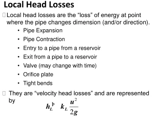
Local Head Losses • Local head losses are the “loss” of energy at point where the pipe changes dimension (and/or direction). • Pipe Expansion • Pipe Contraction • Entry to a pipe from a reservoir • Exit from a pipe to a reservoir • Valve (may change with time) • Orifice plate • Tight bends • They are “velocity head losses” and are represented by
Value of kL • For junctions and bends we need experimental measurements • kL may be calculated analytically for • Expansion • Contraction • By considering continuity and momentumexchangeandBernoulli
Losses at an Expansion • As the velocity reduces (continuity) • Then the pressure must increase (Bernoulli) • So turbulence is induced and head losses occur Turbulence and losses
Value of kL for Expansion • Apply the momentum equation from 1 to 2 1 2 • Using the continuity equation we can eliminate Q • From Bernoulli
Value of kL for Expansion • Combine and - Borda-Carnot Equation • Using the continuity equation again
Losses at Contraction • Flow converges as the pipe contracts • Convergence is narrower than the pipe • Due to vena contractor • Experiments show for common pipes • Can ignore losses between 1 and 1’ • As Convergent flow is very stable
Losses at Contraction • Apply the general local head loss equation between 1’ and 2 • And Continuity The value of k depends on In general
kL values Bell mouth Entry T-branch kL= 1.5 kL= 0.1 Sharp Entry/Exit kL= 0.5 T-inline kL=0.4
Pipeline Analysis • Bernoulli Equation • equal to a constant: Total Head, H • Applied from one point to another (A to B) • With head losses
Bernoulli Graphically • Reservoir • Pipe of Constant diameter • No Flow A
Bernoulli Graphically • Constant Flow • Constant Velocity • No Friction A
Bernoulli Graphically • Constant Flow • Constant Velocity • No Friction Change of Pipe Diameter A
Bernoulli Graphically • Constant Flow • Constant Velocity • With Friction A
Reservoir Feeding Pipe Example • Apply Bernoulli with head losses pA=pC = Atmospheric uA = negligible
Find pressure at B: Apply Bernoulli A-B pA= Atmospheric u = uB = 2.41 m/s Negative i.e. less than Atmospheric pressure
Pipes in series • Consider the situation when the pipes joining two reservoirs are connected in series 1 2 • Total loss of head for the system is given as A1U1=A2U2=AnUn=Q Q1=Q2=Qn=Q
Pipes in Series Example • Two reservoirs, height difference 9 m, joined by a pipe that changes diameter. For, 15m d=0.2 m then for 45 m, d=0.25 m. f = 0.01 for both lengths. • Use kL,entry= 0.5, kL,exit = 1.0. Treat the joining of the pipes as a sudden expansion. • Find the flow between the reservoirs.
Pipes in parallel • The head loss across the pipes is equal • Diameter, f, length L,Q, andu may differ • Total flow is sum in each pipe
Knowing the loss of head, the discharges in each pipe can be obtained • The values of U1, U2 and U3 may be obtained from the above equations and hence the discharges Q1, Q2 and Q3 obtained.
The discharge Q is given, the distribution of discharge in different branches is required • The discharges Q1, Q2, Q3 can be expressed in terms of H Where
Similarly Therefore: As the discharge is known and K1,K2 and K3 are constants, the value of H is obtained and the discharge in individual pipes obtained
Pipes in Parallel Example • Two pipes connect two reservoirs which have a height difference of 10 m. Pipe 1 has diameter 50 mm and length 100 m. Pipe 2 has diameter 100 mm and length 100 m. Both have entry loss kL,entry = 0.5 and exit loss kL,exit =1.0 and Darcy f of 0.008. • Find Q in each pipe • Diameter D of a pipe 100 m long and same f that could replace the two pipes and provide the same flow.
Flow required in new pipe = • Replace u using continuity Must solve iteratively
Must solve iteratively for D • Get approximate answer by leaving the 2nd term • Increase deqa little, say to 0.106 • … a little more … to 0.107 So
Flow through a by-pass • A by-pass is a small diameter pipe connected in parallel to the main pipe Meter By-pass Main pipe The ratio of q in the by-pass, to the total discharge is known as theby-pass coefficient. by-pass coefficient
Head loss in main pipe = head loss in by-pass Minor losses in the by-pass due to bend and the meter etc Divide by Implies
Using continuity equation Adding one on both sides
By-pass coefficient • Knowing the by-pass coefficient, the total discharge in the main pipe can be determined