Estimation

1. Estimation Chapter 10

2. Introduction • Statistical inference is the process by which we acquire information about populations from samples. • There are two procedures for making inferences: • Estimation. • Hypotheses testing.

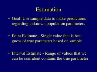
3. The Concepts of Estimation • The objective of estimation is to determine the value of a population parameter on the basis of a sample statistic. • There are two types of estimators: Point Estimator, Interval estimator.

4. Point Estimator A point estimator draws inference about a population by estimating the value of an unknown parameter using a single value or a point.

5. The parameter value Population distribution ? Point estimator Point Estimator A point estimator draws inference about a population by estimating the value of an unknown parameter using a single value or a point. isunknown. The sample statistic is used as a point estimator. Sample distribution S a m p l e

6. We estimate it’s value by providingan interval where it is likely to be found. Population distribution Sample distribution ? Interval Estimator • An interval estimator draws inferences about a population by estimating the value of an unknown parameter using an interval. The parameter is unknown. S a m p l e Interval estimator

7. Insight: Estimator’s Characteristics • Selecting the right sample statistic to estimate a parameter value depends on the statistic characteristics. • Estimator’s desirable characteristics: • Unbiasedness: An unbiased estimator is one whose expected value is equal to the parameter it estimates. • Consistency: An unbiased estimator is said to be consistent if the difference between the estimator and the parameter grows smaller as the sample size increases. • Relative efficiency: For two unbiased estimators, the one with a smaller variance is said to be relatively efficient.

8. With this sample mean, the population mean m is expected to be neither too far below, nor too far above 100. Thus, we construct an interval around 100, where it is likely to find the parameter m. Understanding the Concept of an Interval Estimator for the Mean • To estimate m, a sample of size n is drawn from the population, and its mean is calculated. Let’s assume the sample mean is equal to 100.

9. Understanding the Concept of an Interval Estimator for the Mean The idea is to have the lower bound of the interval determined such that there is a large probability it is smaller than the parameter estimated, and… … to have the upper bound of the interval determined such that there is a large probability it is larger than the parameter estimate. Click to see a demonstration.

10. P( ³100) m Understanding the Concept of an Interval Estimator for the Mean This is the probability the sample mean is at least 100, when the population mean is located at m. Click 100 Assume the sample mean is 100, and the population mean is m.

11. At a certain point (when m = m1) P(³100) is very small, so it is unlikely mshould be shifted to the left any more. In other words m seems to be greater than m1, given . m Understanding the Concept of an Interval Estimator for the Mean m1 £m P( ³100) m1 100 Note how this probability grows smaller if m were smaller (i.e. shifted to the left). Click

12. m2 m P( £100) m1 £m m£m2 m 100 This is the probability to have the sample mean appear at 100 or below, when the population mean is located at m. Click. Note how this probability grows smaller as m is shifted to the right. Click At a certain point when m = m2 we decide that it is unlikely to have m >m2,given the value of the sample mean.

13. 10.2 Estimating the Population Mean when s is known • How is an interval estimator produced from a sampling distribution? • A sample of size n is drawn from the population, and its mean is calculated. • By the central limit theorem, we have established before that…

14. Switching m and we have the relationship The confidence interval 10.2 Estimating the Population Mean when s is known

15. (1 – a)% of all the values of obtained in repeated sampling from a given distribution, construct an interval that includes (covers) the population mean. Interpreting the Confidence Interval for m

16. za/2 1 – a .90 a/2=.05 a/2=.05 .95 .45 Estimation of the Population Mean: known s • Four commonly used confidence levels The probability .95 translates to an entry of .45 in the Z-table, and thus is associated with Z.05 = 1.645. Za/2 = 1.645

17. The mean values obtained in repeated draws of samples of size 100 result in interval estimators of the form [sample mean - .28, Sample mean + .28], 90% of which cover the real mean of the distribution. Estimation of the Population Mean: known s • Example 1: Estimate the mean value of the distribution resulting from the roll of a fair die. It is known that s = 1.71. Use 90% confidence level, and 100 repeated throws of the die • Solution: The confidence interval is

18. Estimation of the Population Mean: known s • Recalculate the confidence interval for 95% confidence level. • Solution:

19. Estimation of the Population Mean: known s • The 90% confidence interval = • The 95% confidence interval = • Because the 95% confidence interval is wider, it is more likely to include the value of m. .95 .90

20. Estimation of the Population Mean: known s • Example 2 • Doll Computer Comp. delivers computers directly to its customers who order via the internet. • To reduce inventory costs in its warehouses Doll employs an inventory model, that requires the estimate of the mean demand during lead time. • It is found that lead time demand is normally distributed with a standard deviation of 75 computers per lead time. • Estimate the lead time demand at 95% confidence level.

21. Additional example Estimation of the Population Mean: known s • Example 2– Solution • The parameter to be estimated is m, the mean demand during lead time. • We need to compute the interval estimation for m. • From the data provided in the file Doll, the sample mean is Since 1 - a =.95, a = .05. Thus a/2 = .025. Z.025 = 1.96

22. Information and the Width of the Interval Comparing two confidence intervals with the same levelof confidence, the narrower interval provides moreinformation than the wider interval Same confidence level!

23. What affects the Width of the Confidence Interval? • The width of the confidence interval is calculated by • and therefore is affected by • the population standard deviation (s) • the confidence level (1-a) • the sample size (n).

24. a/2 a/2 Changing the standard deviation If the standard deviation grows larger, a longer confidence interval is needed to maintain the confidence level. Note what happens when s increases to 1.5s 1-a Confidence level

25. a/2 = 5% a/2 = 2.5% a/2 = 5% a/2 = 2.5% 95% Changing the confidence level Larger confidence level requires longer confidence interval 90% Confidence level

26. Changing the sample size There is an inverse relationship between the width of the interval and the sample size By increasing the sample size we can decrease the width of the confidence interval while theconfidence level can remain unchanged.

27. W 10.3 Selecting the Sample size • The phrase “estimate the mean to within W units”, translates to an interval estimate of the formwhere W is the margin of error. W =

28. 10.3 Selecting the Sample size • The required sample size to estimate the mean is

29. 10.3 Selecting the Sample size • Example 4 • To estimate the amount of lumber that can be harvested in a tract of land, the mean diameter of trees in the tract must be estimated to within one inch with 99% confidence. • What sample size should be taken? (assume diameters are normally distributed with s = 6 inches).

30. If the standard deviation is really 6 inches, the interval resulting from the random sampling will be of the form . If the standard deviation is greater than 6 inches the actual interval will be longer than +/-1. 10.3 Selecting the Sample size • Solution • The margin of error is +/-1 inch. That is W = 1. • The confidence level 99% leads to a = .01, thus za/2 = z.005 = 2.575. • We compute