Le Satellite Odin
Le Satellite Odin. Philippe Ricaud Laboratoire d’Aérologie, Toulouse. 1- Le satellite Odin 2- Spectroscopie dans le domaine sub-mm 3- Validation 4- Résultats scientifiques 5- Implication d’ETHER. Plan. Le satellite Odin. Mini-satellite Suède, France, Canada et Finlande

Le Satellite Odin
E N D
Presentation Transcript
Le Satellite Odin Philippe Ricaud Laboratoire d’Aérologie, Toulouse
1- Le satellite Odin2- Spectroscopie dans le domaine sub-mm3- Validation4- Résultats scientifiques5- Implication d’ETHER Plan
Le satellite Odin • Mini-satellite • Suède, France, Canada et Finlande • 50 % aéronomie, 50% astronomie • 250 kg • 620 km d’altitude, héliosynchrone (18:00 nœud ascendant) • Couverture en latitude : 83°S-83°N • 2 instruments : • Micro-onde (SMR): 480-580 GHz • O3 et isotopes, ClO, N2O, HNO3, H2O et isotopes, CO,température • UV/VIS et IR (OSIRIS): 200-700 nm et 1.27 mm • O3, NO2, aérosols, (BrO, OClO) • Lancement en février 2001 (lanceur START-1)
Géométries d’observation Hauteur tangente Visée au limbe
Le satellite Odin • Configuration “lancement” (replié)
L’instrument SMR • Mélangeurs Schottky refroidis mécaniquement • 4 bandes (480-580 GHz non continues) • A1 541 - 558 GHz • B2 547 - 564 GHz • A2 486 - 504 GHz • B1 563 - 580 GHz • Spectromètres • 2 auto-corrélateurs • 1 spectromètre acousto-optique • 1 banque de filtres (119 GHz pour O2 ® température)
Modes de Mesure • 4 modes scientifiques • Stratosphérique: O3, ClO, HNO3, N2O • Hydrogène : H2O, H2O2, HO2, CO, O3 • Azote: NO, NO2, HNO3, N2O, O3 • Isotope vapeur d ’eau : H2O, HDO, H2O-18, H2O-17, O3 • 3 modes d’observation • Stratosphère : 10-60 km • Strato-mésosphère : 20-70 km • Mésosphère d’été : 60-100 km
MOLIERE : Transfert Radiatif • MOLIERE : Microwave Odin Line Estimation and Retrieval • 0-3 THz • Raie par raie • Visées • Limbe • Nadir • Instruments : sol, ballon-avion & espace • Continua H2O & O2 • Bases de données spectroscopiques JPL & HITRAN • Fonctions de poids instrumentales • Lobe d’antenne • Réponse spectromètres • Modes SSB & DSB
MOLIERE : Retrieval code Estimate the vertical profiles of the studied molecules from the measured spectra • OEM Method (Optimal Estimation Method, Rodgers) • Linearisation of the radiative transfer equation around a reference state xref F(x,b) = F(xref , b) + K|xref(xref –xa) , withK =∂F/∂x • Statistical Combinaison of the information coming from an a priori knowledge xa of the profile and from the measurement y ; weighted by the errors • Least-squared methode : • Minimisation of 2 = [y – F(x, b)]T Sy–1 [y – F(x,b)] + [x – xa] Sa–1 [x – xa] y : measurement ; x : vertical profile ; F : model ; b : model parameters • Sa and Sy: covariance matrix associated with xa and y • Solution given by (Rodgers, 1976) : • x = xa + (Sa–1 + KTSy–1K)–1 KTSy–1 [ y – F(xref , b) + K(xref –xa) ]
Non-linear Retrieval Use the OEM even when the problem is non-linear Solutions 1) Treat only the channels that are optically thin 2) Use a non-linear scheme Iterative scheme based on a Newton and Levenberg-Marquardt iteration • xi+1 = xa + (Sa–1 + KiTSy–1Ki + I)–1 • KTSy–1 [ ( y – F(xi , b) + K(xi – xa) ) + (xi –xa) ] : Levenberg-Marquardt parameter regularisation of the problem solution not too far of the a priori
TRAITEMENT NIVEAU 1B MISU PDC Exogen Data IDRIS L2/OSIRIS L1B/SMR L2/SMR L2/SMR T-P/ECMWF ACQUISITION T-P using ARLETTY Spectra in L1B STORAGE MOLIERE CTSO L2/MOLIERE ETHER CTSO/NOMINAL USERS FRENCH AERONOMERS CTSO/DEVELOPMENT OBSERVATOIRE DE BORDEAUX
Odin/SMR Measurements Studied Molecules and Expected Retrieval
Implication Française Aéronomie • Laboratoires • Observatoire de Bordeaux → Laboratoire d’Aérologie • Service d’Aéronomie • Météo-France/CNRM • Ether, base de données • IPSL (Paris) • CNES (Toulouse) • Chaîne de traitement des données micro-ondes, modélisation, assimilation, interprétation
O3, ClO, N2O Urban et al., 2006
ClO N2O O3 Urban et al., 2006
O3, HNO3 Urban et al., 2006
O3 HNO3 Urban et al., 2006
H2O et isotopes Urban et al., 2007
Vapeur d’eau H2O H2O-18 HDO H2O Urban et al., 2007
CO Dupuy et al., 2005
H2CO Ricaud et al., 2007
Weak Line Studies Zelinger et al., 2007
SAOZ-MIR, SMR and OSIRIS Mean, difference and standard deviation at 22°S (Brasil to Australia) in February 2003 • OSIRIS : within1% and 100 m on average with SAOZ, larger 8% standard dev. 8% in the stratosphere, degrading rapidly below 19 km • SMR: within 7% and 1 km with SAOZ, 20% standard dev. In the stratosphere, degrading below 20 km
N2O : SMR vs LPMA SMR LPMA
O3 N2O ClO O3 ClO N2O 19-20/09/02 25-26/09/02 1-2/10/02 4-5/10/02 REPROBUS Odin Ricaud et al., 2005
Trou d’ozone arctique El Amraoui et al., 2008
N2O ODIN QBO Phase E W E W E MOCAGE SLIMCAT Ricaud et al., 2009
N2O : AO, SAO and QBO Model underestimation of the AO in the UTLS AO SAO QBO Ricaud et al., 2009 Non-negligible measured SAO at 100 hPa
MAM season OPF Overshooting Probability Function (Liu and Zipfser, JGR, 2005) OLR • At 400 K, all measured gases (N2O, CH4 and CO) show significant longitudinal variations, not captured by the model (Ricaud et al., ACP, 2007). • The maximum amounts are primarily located over Africa in MAM 2002-2004. • The suggestion is of strong overshooting over land convective regions, particularly Africa, very consistent with the TRMM maximum overshooting features over the same region during the same season. ODIN N2O 400 K 400 K MOCAGE N2O
1.2 ppbv/yr ; 0.4 ppbv/yr 1.9 ppbv/yr ; 0.2 ppbv/yr 1.7 ppbv/yr ; 1.6 ppbv/yr -3.2 ppbv/yr; -6.3 ppbv/yr 1.6 ppbv/yr ; 1.2 ppbv/yr -0.7 ppbv/yr 1.2 ppbv/yr 0.8 ppbv/yr ; 0.7 ppbv/yr
Exploitation des données ODIN dans ETHER • État de l’archive : • Données SMR : • L1B de 2001 à 2009, V6 : toutes bandes confondues, rapatriement des données de la V7 en cours • L2 non officielles de 2001 à 2008 produites par la CTSO, V225 : molécules N2O, O3 et ClO • L2 officielles V2.1 : de 2001 à 2009 (O3, N2O, ClO) • Données OSIRIS : • L2 de 2001 à 2009, V3.0: O3, NO2 • Exploitation des données ODIN/SMR • Traitement systématique des mesures de N2O, O3 et ClO de l’instrument ODIN/SMR sur Ether • Données 2004 à 2008 produites • Données 2002 (mars – avril –mai ) et 2009 en cours de production • Création et mise à jour des fichiers logs dressant la liste des L1B récupérés et des L2 produits sur Ether
Synthèse • ODIN toujours opérationnel • Mode 100% aéronomie depuis 2007 • Bilan publications ODIN : 127 • SMR : 68 dont 31 françaises, le reste venant de Suède, USA, et Japon • OSIRIS : le reste, essentiellement Canada