Download
1 / 40
400 likes | 417 Vues
This presentation provides updates on the refinement of the MODIS atmospheric correction algorithm by Menghua Wang and Wei Shi, covering topics such as cloud masking, aerosol identification, and SWIR band usage for coastal regions. Work progress and algorithm modifications are discussed.

E N D
Refinement of MODIS Atmospheric Correction Algorithm Menghua Wang (PI, NASA NNG05HL35I) NOAA/NESDIS/ORA Camp Springs, MD 20746, USA Support from: Wei Shi UMBC, NOAA/NESDIS/ORACamp Springs, MD 20746, USA The Ocean Color Research Team Meeting April 11-13, 2006, Hyatt Regency Newport, Newport, Rhode Island
Status of the Algorithm Modifications and Refinements • 1. Wang, M. and W. Shi, “Estimation of ocean contribution at the MODIS near-infrared wavelengths along the east coast of the U.S.: Two case studies,” Geophys. Res. Lett., 32, L13606, doi:10.1029/2005GL022917 (2005). • 2. Wang, M. and W. Shi, “Cloud masking for ocean color data processing in the coastal regions,” IEEE Trans. Geosci. Remote Sens. (Accepted). Status:Developed cloud masking using MODIS SWIR bands (1240/1640/2130 nm). Scheme can be easily implemented into the MODIS data processing system. • 3. Developed schemes to identify cases for the strongly absorbing aerosols and turbid waters with the MODIS SWIR and visible data. Status:A poster is presented in this meeting. Work is in progress. • 4. Atmospheric correction using the MODIS SWIR bands. Status:This presentation. Work is in progress. • 5. Deriving the MODIS high spatial resolution ocean color data. Status:This presentation. Work is in progress.
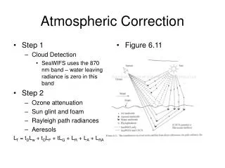
Atmospheric Correction MODISand SeaWiFS algorithm (Gordon and Wang 1994) • wis thedesired quantity in ocean color remote sensing. • Tgis the sun glint contribution—avoided/masked/corrected. • Twcis the whitecap reflectance—computed from wind speed. • risthe scattering from molecules—computed using the Rayleigh lookup tables (atmospheric pressure dependence). • A = a+rais the aerosol and Rayleigh-aerosol contributions —estimated using aerosol models. • For Case-1 waters at the open ocean,wis usually negligibleat750 & 865 nm. A can be estimated using these two NIR bands. Ocean is usually not black at NIR in coastal regions. Gordon, H. R. and M. Wang, “Retrieval of water-leaving radiance and aerosol optical thickness over the oceans with SeaWiFS: A preliminary algorithm,” Appl. Opt., 33, 443-452, 1994.
Atmospheric Correction: SWIR Bands • At the short wave IR (SWIR) wavelengths (>~1000 nm), ocean water has much strongly absorption and ocean contributions are significantly less. Thus, atmospheric correction can be carried out for coastal regions without using the bio-optical model. • Water absorption for 869 nm, 1240 nm, 1640 nm, and 2130 nm are 5 m-1, 88 m-1, 498 m-1, and 2200 m-1, respectively. • Results from simulations were presented in the Hawaii Ocean Science Meeting in Feb. of 2004. • Examples using the MODIS Aqua 1240 and 2130 nm data to derive the ocean color products are provided. • We use the SWIR band (1240 nm) for the cloud masking. This is necessary for coastal region waters.
MODIS Terra Granule:20040711515 (March 11, 2004) The Rayleigh-Corrected TOA Reflectance 748 nm 869 nm 1240 nm 1640 nm Rayleigh-Removed
Data Processing Using the SWIR Bands Software Modifications: • Atmospheric correction package has been significantly modified based on SeaDAS 4.6. • Data structure and format of aerosol lookup tables and diffuse transmittance tables have been changed. • With these changes, it is flexible now to run with different aerosol models (e.g., absorbing aerosols) and with various band combinations for atmospheric correction. Lookup Tables Generation and Implementation: • Rayleigh lookup tables for the SWIR bands (for MODIS 16 bands). • Aerosol optical property data (scattering phase function, single scattering albedo, extinction coefficients) for the SWIR bands (12 models & 16 bands). • The vectoraerosol lookup tables (including the polarization effects) (12 aerosol models) for the SWIR bands, and for the MODIS high-spatial resolution bands. • Table structures are completely changed (different from the current ones). Data Processing: • Regenerated MODIS L1B data including all SWIR band data (for SeaDAS). • Developed cloud masking using the MODIS 1240/1640/2130 nm band. • Aqua-MODIS 15 bands: 412, 443, 469, 488, 531, 551, 555, 645, 667,678,748, 859, 869, 1240, and 2130 nm.
We have carried out vicarious calibration using a MOBY scene from the standard processing…… Vicarious Gains We will use the MOBY in situ measurements for vicarious calibration.
Initial Results We compare the current MODIS results (downloaded directly from Web) and results from algorithmusing SWIR bands. Normalized water-leaving radiances are derived for 412, 443, 469, 488, 531, 551, 555, 645, 667, 678, 748, 859, and 869 nm. High spatial resolution products are derived for nLw(469) and nLw(555) (0.5 km) and nLw(645) and nLw(859) (0.25 km).
Chlorophyll-a (2004096.1820) Standard Processing (748, 869 nm) New Processing (1240, 2130 nm) Absorbing Aerosols April 6, 2004
nLw(443) (2004096.1820) Standard Processing (748, 869 nm) New Processing (1240, 2130 nm) Absorbing Aerosols April 6, 2004
nLw(531) (2004096.1820) Standard Processing (748, 869 nm) New Processing (1240, 2130 nm) April 6, 2004
Noise Effects: Chl-a (2004096.1820) New Processing (SWIR 1 km) New Processing (SWIR 3 km) April 6, 2004
Noise Effects: nLw(531) (2004096.1820) New Processing (SWIR: 1 km) New Processing (SWIR: 3 km) April 6, 2004
Ocean NIR Contributions (SWIR: 3 km) nLw(748) nLw(869) April 6, 2004
Outer Banks Outside of Outer Banks HistogramnLw(443) (2004096.1820) Standard Processing (748, 869 nm) New Processing (1240, 2130 nm) April 6, 2004
Outer Banks Outside of Outer Banks HistogramnLw(488) (2004096.1820) Standard Processing (748, 869 nm) New Processing (1240, 2130 nm) April 6, 2004
Outer Banks Outside of Outer Banks HistogramnLw(531) (2004096.1820) Standard Processing (748, 869 nm) New Processing (1240, 2130 nm) April 6, 2004
Histogram Chl-a in Outer Banks(2004096.1820) Standard Processing (748, 869 nm) New Processing (1240, 2130nm) April 6, 2004
MODIS High Spatial Resolution Measurements Lt(645) (0.25 km) Lt(645) (0.25 km)
High Spatial Resolution Product nLw(645) (1 km, SWIR:1 km) nLw(645) (0.25 km, SWIR:0.5 km) Chesapeake Bay
High Spatial Resolution Product nLw(555) (1 km, SWIR:1 km) nLw(555) (0.5 km, SWIR:0.5 km)
High Spatial Resolution Product nLw(469) (1 km, SWIR:1 km) nLw(469) (0.5 km, SWIR:0.5 km)
High Spatial Resolution Product nLw(645) (1 km, SWIR:1 km) nLw(645) (0.25 km, SWIR:0.5 km) Outer Banks
High Spatial Resolution Product nLw(555) (1 km, SWIR:1 km) nLw(555) (0.5 km, SWIR:0.5 km)
High Spatial Resolution Product nLw(469) (1 km, SWIR:1 km) nLw(469) (0.5 km, SWIR:0.5 km)
High Spatial Resolution ProductnLw(859)(0.5 km, SWIR: 0.5 km)
High Spatial Resolution Product nLw(859) (0.25 km, SWIR:0.5 km) nLw(859) (0.25 km, SWIR:0.5 km)
nLw(645) Ocean Spectrum from Visible to NIR for Various Ocean Waters E D B A C
Conclusions • For the turbid waters in coastal regions, ocean is not black at the NIR bands. This leads to underestimation of the sensor-measured water-leaving radiances with current SeaWiFS/MODIS atmospheric correction algorithm. • Ocean is black for turbid waters at wavelengths >~1000 nm, e.g., 1240 and 2130 nm. Thus, the SWIR bands can be used for atmospheric correction over the turbid waters. No ocean model is needed! • For turbid waters, the Red-NIR nLw contributions are significant and can be useful to derive ocean properties in coastal regions. • To obtain high quality ocean color products, sensor with high (adequate) SNR values is crucial. • Future ocean color sensor needs to include wavelengths > ~1000 nm with high SNR values. • Future works: Calibration/Validation, Dealing with absorbing aerosols, some other details.
High Spatial Resolution Product (SWIR 3 km) nLw(645) (1 km) nLw(645) (0.25 km)
High Spatial Resolution Product (SWIR 3 km) nLw(555) (1 km) nLw(555) (0.5 km)
High Spatial Resolution Product (SWIR 3 km) nLw(645) (1 km) nLw(645) (0.25 km)
Chesapeake Bay Outside of Chesapeake Bay HistogramnLw(443) (2004096.1820) Standard Processing (748, 869 nm) New Processing (1240, 2130 nm) April 6, 2004
Chesapeake Bay Outside of Chesapeake Bay HistogramnLw(488) (2004096.1820) Standard Processing (748, 869 nm) New Processing (1240, 2130 nm) April 6, 2004
Chesapeake Bay Outside of Chesapeake Bay HistogramnLw(531) (2004096.1820) Standard Processing (748, 869 nm) New Processing (1240, 2130 nm) April 6, 2004