Download
1 / 25
250 likes | 339 Vues
An overview of analyzing binary outcomes in research, methods like Adjusted Means Computation, and interpreting Relative Risks with examples.

E N D
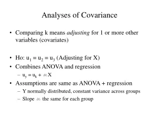
Analyses of Covariance • Comparing k means adjusting for 1 or more other variables (covariates) • Ho: u1 = u2 = u3 (Adjusting for X) • Combines ANOVA and regression • uy = uk + bX • Assumptions are same as ANOVA + regression • Y normally distributed, constant variance across groups • Slope b the same for each group
SAS Code PROCGLM; CLASS group; MODEL chol12 = group cholbl/SS3SOLUTION; MEANS group; LSMEANS group; ESTIMATE‘Adjusted Mean Dif' group 1 -1; RUN;
Adjusted Means ComputationObservations • YBAR(A)i = YBARi – b (XBARi – XBAR) • If b = 0 then adjusted mean equals unadjusted mean • If mean of X is same for all group then adjusted mean equals unadjusted mean
Computing the Adjusted Means • 12-mo Avg. Baseline Avg. • Diuretic 231.7 230.7 • Placebo 219.7 224.9 • Total 227.0 • =0.894 Regression slope of 12-month cholesterol on baseline cholesterol • YBAR(A) (Diur) = 231.7 – 0.894 (230.7 – 227.0) • = 231.7 – 0.894 (3.7) = 228.4 • YBAR(A) (Plac) = 219.7 – 0.894 (224.9 – 227.0) • = 219.7 – 0.894 (-3.7) = 221.6 6.8
Summary of Analyses of Continuous Variables • Y is continuous variable • Estimate a single mean m • Compare 2 means m1 - m2 • Compare k means m1, m2, m3, … mk • Model means as function of 1 or more variables (LR) • Y = b0 + b1X1 + b2X2
Summary of Analyses of Continuous Variables • Hypothesis testing • Ho: m = 0 • Ho: m1 = m2 • Ho: m1 = m2 =mk • Ho: bj = 0
Summary of Analyses of Continuous Variables • Confidence intervals
Analyses of Binary Outcomes • Much of bio-medical data relates to analyses of binary outcomes: • Cancer (yes/no) • Survival (yes/no) • Had side-effect (yes/no) • Currently smoke cigarettes • Social Sciences: • Divorced (yes/no) • Return to prison (yes/no) • Political: • Favor a candidate (yes/no) • State has capital punishment (yes/no)
Analyses of Binary Variables • Y has two outcomes (yes/no or 1/0) • Estimate a single proportion p • Compare 2 proportions p1 - p2 • Compare k proportions p1, p2, p3, … pk • Model probability as function of 1 or more variables • Y = b0 + b1X1 + b2X2
Binary Outcomes • Binary outcomes (Y=0 or 1) can be thought of in terms of probabilities: P (Y=1) = p P (Y=0) = (1 – p) • The ratio of the P(Y=1) to P(Y=0) is the odds O = Odds (Y=1 versus Y = 0) = P(Y=1)/P(Y=0) = p /(1 – p)
Example • Y = 1 indicates your horse winning the race P (Y=1) = 0.20 P (Y=0) = (1 – 0.20) = 0.80 • What is the Odds of winning versus losing. Odds = P(Winning)/P(Losing) = 0.20/0.80 = 0.25 or ¼ In gambling terms the odds are 4 to 1.
Relationship Between Probability and Odds p Odds (o=p/(1-p)) 0.95 19.00 0.50 1.00 0.40 0.67 0.30 0.43 0.20 0.25 0.15 0.18 0.10 0.11 0.05 0.053 0.01 0.0101 For small values the probability and the odds are close in value
Comparing Two Groups With Binary Outcomes p1 = probability of Y=1 for group 1 p2 = probability of Y=1 for group 2 Ways to summarize the probability differences: 1) p1- p2 difference in probabilities 2) p1/ p2 ratio of probabilities (Relative Risk) 3) (p1/(1-p1)/ ratio of odds (Relative Odds) (p2/(1-p2)
Example Group 1: Smokers Group 2: Non-smokers Y = 1 indicates cough upon awakening p1 = 0.30 p2 = 0.20 p1- p2 = 0.10 p1/ p2 = 0.30/0.20 = 1.50 o1/ o2 = (.30/.70)/(.20/.80) = 0.429/0.250 = 1.71
Interpretation of Relative Risks Group 1: Smokers Group 2: Non-smokers • RR = 1.50 • There is a 50% increased risk of cough for smokers compared to non-smokers. • Smokers are at a 50% increased risk of cough compared to non-smokers
Interpretation of Relative RisksChanging the Reference Group Group 1: Non-Smokers Group 2: Smokers • RR = 0.67 (1/1.50 or .20/.30) • There is a 33% decreased risk of cough for non-smokers compared to smokers. • Non-smokers are at a 33% lower risk of cough compared to smokers.
NEJM March 2005: A Randomized Trial of Low-Dose Aspirin in the Primary Prevention of Cardiovascular Disease in Women Results: During follow-up, 477 major cardiovascular events were confirmed in the aspirin group, as compared with 522 in the placebo group, for a nonsignificant reduction in risk with aspirin of 9 percent (relative risk, 0.91; 95 percent confidence interval, 0.80 to 1.03; P=0.13). With regard to individual end points, there was a 17 percent reduction in the risk of stroke in the aspirin group, as compared with the placebo group (relative risk, 0.83; 95 percent confidence interval, 0.69 to 0.99; P=0.04), owing to a 24 percent reduction in the risk of ischemic stroke (relative risk, 0.76; 95 percent confidence interval, 0.63 to 0.93; P=0.009) and a nonsignificant increase in the risk of hemorrhagic stroke (relative risk, 1.24; 95 percent confidence interval, 0.82 to 1.87; P=0.31). As compared with placebo, aspirin had no significant effect on the risk of fatal or nonfatal myocardial infarction (relative risk, 1.02; 95 percent confidence interval, 0.84 to 1.25; P=0.83) or death from cardiovascular causes (relative risk, 0.95; 95 percent confidence interval, 0.74 to 1.22; P=0.68). Gastrointestinal bleeding requiring transfusion was more frequent in the aspirin group than in the placebo group (relative risk, 1.40; 95 percent confidence interval, 1.07 to 1.83; P=0.02).
Relationship Between Relative Risk and Relative Odds • RO = RR x (1-p2) / (1-p1) • If p1 andp2 are small (<0.10) then • RO ~ RR • Because of this relative risk and relative odds are sometimes interpreted in the same way
Example RR = 2.0 and RR=0.5 • RR = 2.0 p1 p2 Odds Ratio 0.20 0.10 2.25 0.10 0.05 2.11 0.05 0.025 2.05 • RR = 0.5 p1 p2 Odds Ratio 0.10 0.20 0.44 0.05 0.10 0.47 0.025 0.05 0.49
Why Use Ratios • In most cases the probability of an event is dependent on length of time p = p (time) • Using ratios removes time as a factor p1(t) = prob. of developing lung cancer for smokers p2 (t)= prob. of developing lung cancer for non-smokers • RR = p1(t) / p2 (t) • Using differences does not remove time as a factor DIF = p1(t) - p2 (t)
Comparing Studies With DifferentFollow-up Time • Study 1 follows patients for 5 years: p1(5) = 0.10 prob. of developing lung cancer for smokers p2 (5)= 0.02 prob. of developing lung cancer for non-smokers • RR = 0.10/0.02 = 5 • Study 2 follow patients for 30 years: p1(30) = 0.40 prob. of developing lung cancer for smokers p2 (30)= 0.08 prob. of developing lung cancer for non- smokers • RR = 0.40/0.08 = 5
Hypothesis TestingConfidence Intervals • Ho: p1 = p2 • Ha: p1≠p2 • Estimate p1 with p1 = number with condition/total in group 1 • Estimate p2 with p2 = number with condition/total in group 2 • p1-p2 is point estimate of p1 -p2
Proportions for two groups 95% CI for difference in proportions:
Proportions for two groups Example • 50 men with 13 smokers • 50 women with 10 smokers p1 = 13/50 = 0.26, p2 = 10/50 = 0.20 SE = sqrt(0.003848 + 0.0032) = 0.084 95% CI for difference = 0.06 ± 1.96*0.084 0.06 ± 0.165 (-0.105, 0.225) We do not have evidence that the proportion of smokers is different for men and women
Estimation a Single Proportion Example • N=625 sampled; X=# favor • X = 300 p = 300/625 = 0.48 SE = SQRT( (0.48)(0.52)/625) = 0.020 95% CI: = 0.48 ± 1.96*0.02 0.48 ± 0.04 (0.44, 0.52)