Download

1 / 23
240 likes | 448 Vues
Analysis of Covariance. Harry R. Erwin, PhD School of Computing and Technology University of Sunderland. Resources. Crawley, MJ (2005) Statistics: An Introduction Using R. Wiley. Freund, RJ, and WJ Wilson (1998) Regression Analysis, Academic Press.

E N D
Analysis of Covariance Harry R. Erwin, PhD School of Computing and Technology University of Sunderland
Resources • Crawley, MJ (2005) Statistics: An Introduction Using R. Wiley. • Freund, RJ, and WJ Wilson (1998) Regression Analysis, Academic Press. • Gonick, L., and Woollcott Smith (1993) A Cartoon Guide to Statistics. HarperResource (for fun).
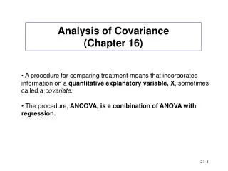
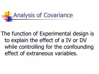
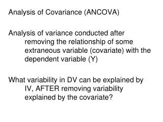
Introduction • Analysis of covariance (ANCOVA) combines regression and ANOVA • Response variable is continuous • One or more explanatory factors (the treatments) • One or more continuous explanatory variables • Usually done in a treatment study where explanatory variables are being included to improve the basic treatment/control comparison. • Interaction between the slope for an explanatory variable and the treatment is not wanted. (Life is hard.) • Maximal model includes estimating slopes and intercepts for each combination of the explanatory factors. • Model simplification is the goal.
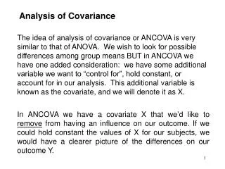
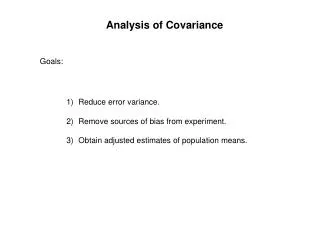
Context • The goal of analysis of covariance is to reduce the error variance. This increases the power of tests and narrows the confidence intervals. • There may be measurable variables that affect the response but have nothing to do with the factors (treatments) in the experiment. • Analysis of covariance adjusts for those variables.
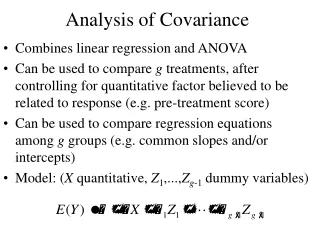
The Covariance Model • For one treatment factor and one continuous control variable, xij, the model is: • yij=0 + i + 1xij + ij • This says the response is a constant (0) plus a second constant (i, depending on the factor) plus a third constant (1) times the control variable (or covariate) plus an error (ij). • The interest is in the difference between the treatment means (the i), not in the 0 or 1. You want to be able to reduce your model.
Assumptions in ANCOVA • The covariate xij is not affected by the experimental factors. • The regression relationship measured by 1 must be the same for all factor levels. You need to verify these assumptions.
General Approach to ANCOVA • First look at the effect of xij. If it isn’t significant, do an ANOVA and be done with it. • Check to see that xij is not significantly affected by the factor values. • Test to see that 1 is not significantly different for all factor levels. This is an interaction (a bad thing) between the factors and the covariates. • Order matters: the covariates come after the factors in the model because they’re less important. • If both tests pass, do the ANCOVA.
Example • Response variable is weight • Explanatory factor is sex • Continuous explanatory variable is age. • weightmale = amale + bmale age • weightfemale = afemale + bfemale age • Six possible models. • The goal is to eliminate as many parameters as possible. • Reduce the model until all parameters are significant.
Book Example • Notes • Use of plots to get insight into the significance of explanatory variables. • Note use of lm() in the models. It produces the same results as aov(), but with a different report. • Order matters—non-orthogonal data! • Use of summary.aov() • Eliminate interactions first. • anova() used in comparisons. • summary.lm() to provide the parameter estimates
Background • This experiment studies the ability of a plant to regrow and produce seeds after grazing. • The pregrazing size is the diameter of the top of the rootstock • Grazing has two levels: grazed or ungrazed. • Response is weight of seeds produced at the end of the growing season. • Size of plant is believed to matter and also whether it was grazed.
Step 1 compensation<-read.table("compensation.txt",header=T) attach(compensation) names(compensation) [1] "Root" "Fruit" "Grazing” par(mfrow=c(2,2)) plot(Root,Fruit) plot(Grazing,Fruit)
Step 2 model<-lm(Fruit~Root*Grazing)wrong way--inflates Grazing sum of sqs! summary.aov(model) Df Sum Sq Mean Sq F value Pr(>F) Root 1 16795.0 16795.0 359.9681 < 2.2e-16 *** Grazing 1 5264.4 5264.4 112.8316 1.209e-12 *** Root:Grazing 1 4.8 4.8 0.1031 0.75 Residuals 36 1679.6 46.7 model<-lm(Fruit~Grazing*Root)correct way! Grazing is more important. summary.aov(model) Df Sum Sq Mean Sq F value Pr(>F) Grazing 1 2910.4 2910.4 62.3795 2.262e-09 *** Root 1 19148.9 19148.9 410.4201 < 2.2e-16 *** Grazing:Root 1 4.8 4.8 0.1031 0.75 Residuals 36 1679.6 46.7
Check to see if the interaction term is important model2<-lm(Fruit~Grazing+Root) anova(model,model2)use anova to compare models Analysis of Variance Table Model 1: Fruit ~ Grazing * Root Model 2: Fruit ~ Grazing + Rootsimpler model Res.Df RSS Df Sum of Sq F Pr(>F) 1 36 1679.65 2 37 1684.46 -1 -4.81 0.1031 0.75
Report summary.lm(model2) Coefficients: Estimate Std. Error t value Pr(>|t|) (Intercept) -127.829 9.664 -13.23 1.35e-15 *** GrazingUngrazed 36.103 3.357 10.75 6.11e-13 *** Root 23.560 1.149 20.51 < 2e-16 *** Residual standard error: 6.747 on 37 degrees of freedom Multiple R-squared: 0.9291, Adjusted R-squared: 0.9252 F-statistic: 242.3 on 2 and 37 DF, p-value: < 2.2e-16 Row 1 is the intercept for the factor level first in the alphabet (Grazed as opposed to Ungrazed). Row 2 is the difference Ungrazed – Grazed. Row 3 is the slope of the graph of seed production against rootstock size. Row 4 (when present) is the difference in slopes if the interaction term is significant. (Not significant here! 8)
What’s Going On? sf<-split(Fruit,Grazing) sr<-split(Root,Grazing) plot(Root,Fruit,type="n",ylab="Seed production",xlab="Initial root diameter") points(sr[[1]],sf[[1]],pch=16) points(sr[[2]],sf[[2]]) plot(Root,Fruit,type="n",ylab="Seed production",xlab="Initial root diameter") points(sr[[1]],sf[[1]],pch=16) points(sr[[2]],sf[[2]]) abline(-127.829,23.56) abline(-127.829+36.103,23.56,lty=2)
Suppose we ignored the initial root size? tapply(Fruit,Grazing,mean) Grazed Ungrazed 67.9405 50.8805 the opposite of the true situation! summary(aov(Fruit~Grazing)) Df Sum Sq Mean Sq F value Pr(>F) Grazing 1 2910.4 2910.4 5.3086 0.02678 * Residuals 38 20833.4 548.2 --- Signif. codes: 0 ‘***’ 0.001 ‘**’ 0.01 ‘*’ 0.05 ‘.’ 0.1 ‘ ’ 1
Order Matters for Non-Orthogonal Data! • The total variation in the response (SSY) is equal to the sum of the: • Variation explained by the treatment (SSA), plus the • Variation explained by the covariate, plus the • Variation explained by the interaction between the factor levels and the covariate (hopefully small), plus the • Variation explained by the error term. • Since the factor levels and the covariate are dependent in non-orthogonal data, fitting the covariate first inflates the variation explained by the treatment, potentially producing an invalid positive result. • So put the treatment variable first in the model.
Because Order Matters! • Do you fit the categorical (treatment, T) or the continuous (control, L) explanatory variable first? With non-orthogonal data, order matters. • Use a logical order. Hence fit to the treatment variable first. You’re interested in the effect of the treatment, not of the control variable. • If the interaction between the treatment and control variables is significant, stop! It means the slopes differ significantly, which is a (nasty) problem.
Reading the Summary summary.lm(model2) Call: lm(formula = Fruit ~ Grazing + Root) Residuals: Min 1Q Median 3Q Max -17.1920 -2.8224 0.3223 3.9144 17.3290 Coefficients: Estimate Std. Error t value Pr(>|t|) (Intercept) -127.829* 9.664 -13.23 1.35e-15 *** GrazingUngrazed 36.103** 3.357 10.75 6.11e-13 *** Root 23.560*** 1.149 20.51 < 2e-16 *** Residual standard error: 6.747 on 37 degrees of freedom Multiple R-Squared: 0.9291, Adjusted R-squared: 0.9252 F-statistic: 242.3 on 2 and 37 DF, p-value: < 2.2e-16
Using split() • Applies to a vector or dataframe. • sd<-split(d,f) divides the data in a dataframe (or vector), d, based on the factor, f. • sd will be a list of vectors. Each vector in the list will correspond to a value of the factor (in alphabetical order). • Each vector in sd can be plotted using its own symbol to give insight into the differences between factors. • Book example.
The Moral • If you have covariates, use them. They will improve your confidence intervals or identify that you have a problem. • Order matters—(it always does in regression). • Start by removing the highest order interaction terms first. • Use a logical order. • If the treatment (categorical) interacts significantly with the control (continuous), stop!