Download
1 / 24
240 likes | 526 Vues
Chapter 2: The Process View of an Organization. Process Structures. Continuous Processing Repetitive (assembly lines) Batch processing Job Shops. “continuous or semi-continuous”. “intermittent”. The Product-Process Matrix. Low Volume (unique). Medium Volume (high variety). High Volume

E N D
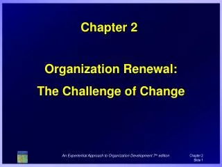
Process Structures Continuous Processing Repetitive (assembly lines) Batch processing Job Shops “continuous or semi-continuous” “intermittent”
The Product-Process Matrix Low Volume (unique) Medium Volume (high variety) High Volume (lower variety) Very high volume (standardized) Unit variable costs generally too high Job Shop CABG Surgery Batch Process Exec. Shirt Manzana Insurance Worker-paced line Toshiba Machine-paced line Toyota Utilization of fixed capital generally too low National Cranberry Continuous process • Categorizes processes into one of five clusters • Similar processes tend to have similar problems • There exists a long-term drift from the upper left to the lower right
Exercise • Form a group of 2-3 students • From your experience/observation, select a product produced for each of these processing models: • Job shop • Batch processing • Assembly line • Continuous processing • Share results with the class
Three Measures of Process Performance Process Inputs Outputs Flow units (raw material, customers) Goods Goods Services Services Resources Labor & Capital Resources Labor & Capital First choose an appropriate flow Unit – a customer, a car, a scooter, etc. • Inventory (WIP in a process) • Flow time • Time it takes a unit to get through the process • Flow rate (throughput rate) • Rate at which the process is delivering output • Maximum rate that a process can generate supply is called the capacity of the process
Little’s Law Patients 11 10 9 8 7 6 5 4 3 2 1 0 Cumulative Inflow Cumulative Outflow Flow Time Inventory Inventory=Cumulative Inflow – Cumulative Outflow Time 7:00 8:00 9:00 10:00 11:00 12:00 13:00 14:00 15:00 16:00 17:00 18:00 What it is: Inventory (I) = Flow Rate (R) * Flow Time (T) Implications: • Out of the three performance measures (I,R,T), two can be chosen by management, the other is GIVEN by nature • Hold throughput (flow rate) constant: Reducing inventory = reducing flow time
Examples Suppose that from 12 to 1 p.m. 200 students per hour enter the GQ and each student is in the system for an average of 45 minutes. What is the average number of students in the GQ? Inventory = Flow Rate * Flow Time = 200 per hour * 45 minutes (= 0.75 hours) = 150 students If ten students on average are waiting in line for sandwiches and each is in line for five minutes, on average, how many students are arrive each hour for sandwiches? Flow Rate = Inventory / Flow Time = 10 Students / 5 minutes = 0.083 hour = 120 students per hour Problem 2.2: Airline check-in data indicate from 9 to 10 a.m. 255 passengers checked in. Moreover, based on the number waiting in line, airport management found that on average, 35 people were waiting to check in. How long did the average passenger have to wait? Flow Time = Inventory / Flow Rate = 35 passengers / 255 passengers per hour = 0.137 hours = 8.24 minutes
Queuing Theory Waiting occurs in Service facility • Fast-food restaurants • post office • grocery store • bank Manufacturing Equipment awaiting repair Phone or computer network Product orders Why is there waiting?
Measures of System Performance • Average number of customers waiting • In the queue (Lq) • In the system (L) • Average time customers wait • In the queue (Wq) • In the system (W) • System utilization (r)
Number of Servers Single Server Multiple Servers Multiple Single Servers
Some Models 1. Single server, exponential service time (M/M/1) 2. Multiple servers, exponential service time (M/M/s) A Taxonomy M / M / s Poisson Arrival Exponential Number of Distribution Service Dist Servers where M = exponential distribution (“Markovian”) (Both Poisson and Exponential are Markovian – hence the “M” notation)
Given l = customer arrival rate m = service rate (1/m = average service time) s = number of servers Calculate Lq = average number of customers in the queue L = average number of customers in the system Wq = average waiting time in the queue W = average waiting time (including service) Pn = probability of having n customers in the system r = system utilization Note regarding Little’s Law: L = l* W and Lq =l * Wq
Model 1: M/M/1 Example The reference desk at a library receives request for assistance at an average rate of 10 per hour (Poisson distribution). There is only one librarian at the reference desk, and he can serve customers in an average of 5 minutes (exponential distribution). What are the measures of performance for this system? How much would the waiting time decrease if another server were added?
Example: One Fast Server or Many Slow Servers? Beefy Burgers is considering changing the way that they serve customers. For most of the day (all but their lunch hour), they have three registers open. Customers arrive at an average rate of 50 per hour. Each cashier takes the customer’s order, collects the money, and then gets the burgers and pours the drinks. This takes an average of 3 minutes per customer (exponential distribution). They are considering having just one cash register. While one person takes the order and collects the money, another will pour the drinks and another will get the burgers. The three together think they can serve a customer in an average of 1 minute. Should they switch to one register?
3 Slow Servers 1 Fast Server W is less for one fast server, so choose this option.
Application of Queuing Theory We can use the results from queuing theory to make the following types of decisions: How many servers to employ Whether to use one fast server or a number of slower servers Whether to have general purpose or faster specific servers Goal: Minimize total cost = cost of servers + cost of waiting
Cost/Benefit Analysis Cost of service: # Servers * Cost of each server Service cost = s * Cs Cost of Waiting: Cost of waiting * Time waiting * number of customers/time unit Waiting Cost = l * Cw * W If you save more in waiting than you spend in service, make the change Example A fast food restaurant has three servers, each earning $10 per hour. Fifty customers per hour arrive and a server can serve a customer in three minutes. Should the restaurant add a fourth server if the cost of a customer waiting is estimated at $20 per hour? Answer
Example: Southern Railroad The Southern Railroad Company has been subcontracting for painting of its railroad cars as needed. Management has decided the company might save money by doing the work itself. They are considering two alternatives. Alternative 1 is to provide two paint shops, where painting is to be done by hand (one car at a time in each shop) for a total hourly cost of $70. The painting time for a car would be 6 hours on average (assume an exponential painting distribution) to paint one car. Alternative 2 is to provide one spray shop at a cost of $175 per hour. Cars would be painted one at a time and it would take three hours on average (assume an exponential painting distribution) to paint one car. For each alternative, cars arrive randomly at a rate of one every 5 hours. The cost of idle time per car is $150 per hour. • Estimate the average waiting time in the system saved by alternative 2. • What is the expected total cost per hour for each alternative? Which is the least expensive? Answer: Alt 2 saves 1.87 hours. Cost of Alt 1 is: $421.25 / hour and cost of Alt 2 is $400.00 /hour.
Calculating Inventory Turns & Per Unit Inventory Costs Annual inventory costs (as a % of item value) include financing costs, depreciation, obsolescence, storage, handling, theft • Obtaining data • Look up inventory value on the balance sheet • Look up cost of goods sold (COGS) from earnings statement – not sales!! • Common benchmark is inventory turns • Inventory Turns = COGS/ Inventory Value • Compute per unit inventory costs: Per unit inventory costs = Annual inventory costs (as a % of item cost) / Inventory turns
Example Problem 2.3: A manufacturing company producing medical devices reported $60 million in sales last year. At the end of the year, they had $20 million worth of inventory in ready-to ship devices. Assuming that units are valued at $1000 per unit and sold at $2000 per unit, what is the turnover rate? Assume the company uses a 25% per year cost of inventory. What is the inventory cost for a $1000 (COGS) item. Assume that inventory turns are independent of price. Answer Sales = $60,000,000 per year / $2000 per unit = 30,000 units sold per year @ $1000 COGS per unit Inventory = $20,000,000 / $1000 per unit = 20,000 units in inventory Turns = COGS/Inventory = $30,000,000/$20,000,000 = 1.5 turns Cost of Inventory: For a $1000 product, the total inventory cost (for one turn) is $1000* 25% or $250. This divided by 1.5 turns gives an absolute inventory cost of $166.66.
Why Hold Inventory? Cumulative Number of patients 7 6 5 4 3 2 1 1.5 Patients 1.5 hours 7:00 8:00 9:00 10:00 11:00 12:00 Time • Pipeline inventory • Seasonal Inventory
Why Hold Inventory? Cumulative Inflow and outflow 1200 1000 Cumulativeinflow 800 Safety inventory 600 400 Cumulativeoutflow 200 0 1 3 5 7 9 11 13 15 17 19 21 23 25 27 29 Days of the month Figure 2.12: Safety inventory at a blood bank • Cycle Inventory • Decoupling inventory/Buffers • Safety Inventory
Inventory Turnover Statistics Retail Hardware stores: 3.5 Retail Nurseries & Garden Supply: 3.3 General Merchandise Stores: 4.7 Grocery Stores: 12.7 New & Used Car Dealers: 6.8 Gas stations & mini-marts: 39.3 Apparel & Accessories: 3.5 Furniture & home furnishings: 4.1 Drug Stores: 5.3 Liquor Stores: 6.6 Other Retail Stores: 4.3 Wholesale Groceries & related: 17.8 Vehicles & automotive: 6.9 Furniture & fixtures: 5.5 Sporting goods: 4.8 Drug store items: 8.5 Apparel & related: 5.5 Petroleum & related: 42.4 Alcoholic beverages: 8.5 Industries with higher gross margins tend to have lower inventory turns Source: Bizstats.com