Advanced Rendering Techniques Using Virtual Light Field (VLF)
This report explores the implementation and rendering methodologies associated with the Virtual Light Field (VLF) project at University College London. It details techniques for rendering ray intersections, applying false color rendering, and overcoming limitations such as resolution blurring. The VLF efficiently handles diffuse textures and specular surfaces through a hybrid approach using OpenGL and ray tracing. Walkthrough results illustrate its performance in achieving global illumination effects in real-time. The report provides insights into future improvements and questions regarding VLF capabilities.

Advanced Rendering Techniques Using Virtual Light Field (VLF)
E N D
Presentation Transcript
Research funded by: Virtual Light Field Group vlfproject@cs.ucl.ac.uk University College London GR/R13685/01 VLF Rendering & Implementation Details Jesper Mortensen j.mortensen@cs.ucl.ac.uk
Overview • Rendering from the VLF • Implementation details • Walkthrough results • Limitations • Future work • Questions
Rendering: VLF • The VLF can be used to render any ray • Determine intersected polygons with false colour rendering • Lookup hemisphere triangle in which direction falls, with barycentric coordinates • In each direction lookup the TRM for the intersected polygon • Interpolate radiance in TRM from 8-neighbourhood • Apply barycentric weights to interpolate the 3 radiances
Rendering: VLF • However, due to limited resolution blurring may occur • Especially for specular surfaces • Expensive:- 3 dirs * 9 TRM cells * rays • Example has 2K directions, 128x128 resolution
Rendering: Diffuse textures • The VLF also stores diffuse maps for any diffuse surface • These can be efficiently rendered using D3D/OpenGL • Limiting blurring to non-diffuse surfaces
Rendering: Backwards ray tracing • Backwards ray tracing can be used for specular parts • Can reconstruct specularly reflected geometry well • Bounces until diffuse surface hit • Can be slow if a large part of the scene is specular
Rendering: Progressive method • Hybrid method • Uses OpenGL texturing for diffuse surfaces • Uses direct VLF lookup for specular surfaces during motion • If viewpoint is stationary renders specular reflection using backwards ray tracing
Implementation: Language • Class based C++ • Heavy use of class templates- flexibility- efficiency, can tailor implementation- con: must recompile
Implementation: Platform • PC based • Windows 2000/XP • Visual Studio .NET
Implementation: Graphics API • Graphics API: OpenGL • Standard pbuffers • Used for ‘false colour’ rendering [visibility]- exchange buffers- rendering phase • Main issue is slow framebuffer readback
Implementation: Libraries • Hierarchical scene graph library- facesets, spheres, blobs etc. • Graphics library- matrices, vectors, materials, cameras etc. • VLF library- tiles, radiance maps, diffuse maps etc.
Implementation: Dependencies • Glut- http://www.opengl.org/developers/documentation/glut/ • Zlib- http://www.gzip.org/zlib/ • Jpeglib- http://www.ijg.org/
Implementation: GI framework • General framework for Global Illumination • Supports many approximations…
Implementation: OpenGL real-time • OpenGL rendering for real-time local illumination
Implementation: Radiosity • Progressive radiosity- Cohen et .al 1988
Implementation: Classic ray tracing • Whitted ray tracing- Turner Whitted 1980
Implementation: Distributed ray tracing • Distributed ray tracing- Robert L. Cook et. al. 1984
Implementation: Path tracing • Coming soon … Monte Carlo path tracing- James T. Kajiya 1986
Implementation: VLFs • And of course – Virtual Light Fields… • Diffuse • Specular • Caustics
Implementation: VLF applications • There are three main applications currently: • VLF analyser- visualises elements of the VLF, PSFs, tiles, maps, visibility etc. good debugging tool • VLF propagator- solves GI for a VLF, outputs binary VLF files, can reload and continue from a binary file • VLF walkthrough- loads a binary VLF file and renders it in real-time
Implementation: HDR viewer • GI results are natively HDR but display devices are inherently LDR [24 bit RGB]! • We have our own file format- similar to Wards radiance format • 32 bit floats RGB interleaved- optionally zip compressed • … and an associated viewer
Implementation: HDR viewer (contd.) • Uses simple linear scaling approaches • Or tone mapping a la Reinhard et. al. 2002
Walkthrough results • The following shows results from walkthroughs of VLFs • The illustrate real-time performance for scenes with global illumination effects • They were all rendered on a dual 2.8 GHZ Pentium 4 Xeon with 3GB RAM, and a NVIDIA GeForce FX5800
Walkthrough results: Cornell scene • This illustrates diffuse GI effects such as colour bleeding and soft shadows • The VLF uses 2K directions and 8x8 tiles each having 16x16 cells • The progressive method is used for rendering
Walkthrough results: Cornell scene SHOW CORNELL VIDEO
Walkthrough results: Office scene • This illustrates GI effects such as specular reflections, soft shadows and colour bleeding • The VLF uses 2K directions and 8x8 tiles each having 16x16 cells • Memory usage is 980MB, propagation time was 36 hrs. • The progressive method and CRT method used for rendering
Walkthrough results: Office scene SHOW PROGRESSIVE OFFICE VIDEO SHOW CRT OFFICE VIDEO
Walkthrough results: GI benchmark • Global illumination test scene from Smits & Jensens repository:- http://www.cs.utah.edu/~bes/papers/scenes/ • Illustrates several interesting light paths: LDE, LDSE, LDSDE (of which the last is a caustic) • The VLF uses 2K directions and 8x8 tiles each having 16x16 cells • Propagation time was 33 hrs. • The progressive method used for rendering
Walkthrough results: GI benchmark SHOW GI BENCHMARK VIDEO
Limitations • Limited to planar geometry • Support for basic materials • No participating media • Closed polyhedra
Whats next? • Investigate alternative rendering methods- Lens approach • Optimise, graphics hardware