Nonparametric Statistics
330 likes | 495 Vues
Nonparametric Statistics. In previous testing, we assumed that our samples were drawn from normally distributed populations. This chapter introduces some techniques that do not make that assumption. These methods are called distribution-free or nonparametric tests.

Nonparametric Statistics
E N D
Presentation Transcript
In previous testing, we assumed that our samples were drawn from normally distributed populations. This chapter introduces some techniques that do not make that assumption. These methods are called distribution-free or nonparametric tests. In situations where the normal assumption is appropriate, nonparametric tests are less efficient than traditional parametric methods. Nonparametric tests frequently make use only of the order of the observations and not the actual values.
In this section, we will discuss four nonparametric tests: the Wilcoxon Rank Sum Test (or Mann-Whitney U test), the Wilcoxon Signed Ranks Test, the Kruskal-Wallis Test, and the one sample test of runs.
The Wilcoxon Rank Sum Testor Mann-Whitney U Test This test is used to test whether 2 independent samples have been drawn from populations with the same median. It is a nonparametric substitute for the t-test on the difference between two means.
Wilcoxon Rank Sum Test Example: Based on the following samples from two universities, test at the 10% level whether graduates from the two schools have the same average grade on an aptitude test.
First merge and rank the grades. Sum the ranks for each sample. rank sum for university A: 74 rank sum for university B: 136 Note: If there are ties, each value gets the average rank. For example, if 2 values tie for 3th and 4th place, both are ranked 3.5. If three differences would be ranked 7, 8, and 9, rank them all 8.
critical region critical region .45 .45 .05 .05 -1.645 0 1.645 Z Since the critical values for a 2-tailed Z test at the 10% level are 1.645 and -1.645, we reject H0 that the medians are the same and accept H1 that the medians are different.
For small sample sizes, you can use Table E.6 in your textbook, which provides the lower and upper critical values for the Wilcoxon Rank Sum Test. • That table shows that for our 10% 2-tailed test, the lower critical value is 82 and the upper critical value is 128. • Since our smaller sample’s rank sum is 74, which is outside the interval (82, 128) indicated in the table, we reject the null hypothesis that the medians are the same and conclude that they are different. • Equivalently, since the larger sample’s rank sum is 136, which is also outside the interval (82, 128), we again reject the null hypothesis that the medians are the same and conclude that they are different.
The Wilcoxon Signed Rank Test This test is used to test whether 2 dependent samples have been drawn from populations with the same median. It is a nonparametric substitute for the paired t-test on the difference between two means.
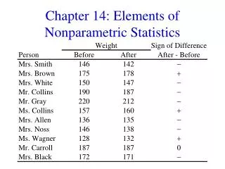
Wilcoxon Signed Rank Test Procedure • Calculate the differences in the paired values (Di=X1i – X2i) • Take absolute values of the differences and rank them (Discard all differences that equal 0.) • Assign ranks Ri with the smallest rank equal to 1. • As in the rank sum test, if two or more of the differences are equal, each difference gets the average rank. (That is, if two differences would be ranked 3 and 4, rank them both 3.5. If three differences would be ranked 7, 8, and 9, rank them all 8.) • Assign the symbol + to positive differences and – to negative differences. • Calculate the Wilcoxon statistic W as the sum of the positive ranks. So,
Example Suppose we have a class with 22 students, each of whom has two exam grades. We want to test at the 5% level whether there is a difference in the median grade for the two exams.
We calculate the difference between the exam grades:diff = exam2 – exam 1.
Then we rank the absolute values of the differences from smallest to largest, omitting the two zero differences. The smallest non-zero |differences| are the two |-1|’s. Since they are tied for ranks 1 and 2, we rank them both 1.5. Since the differences were negative, we put the ranks in the negative column.
The next smallest non-zero |differences| are the two |2|’s. Since they are tied for ranks 3 and 4, we rank them both 3.5. Since the differences were positive, we put the ranks in the positive column.
The next smallest non-zero |differences| are the two |-3|’s and the |3|. Since they are tied for ranks 5, 6, and 7, we rank them all 6. Then we put the ranks in the appropriately signed columns.
We continue until we have ranked all the non-zero |differences| .
Then we total the signed ranks. We get 154 for the sum of the positive ranks and 56 for the sum of the negative ranks. The Wilcoxon test statistic is the sum of the positive ranks. So W = 154.
critical region critical region .475 .475 .025 .025 -1.96 0 1.96 Z Since we had 22 students and 2 zero differences, the number of non-zero differences n = 20. Since the critical values for a 2-tailed Z test at the 5% level are 1.96 and -1.96, we can not reject the null hypothesis H0 and so we conclude that the medians are the same.
For small sample sizes, you can use Table 12.19 in the online material associated with section 12.8 of your textbook, which provides the lower and upper critical values for the Wilcoxon Signed Rank Test. This table is shown on the next slide.
Recall that we have 20 non-zero differences and are performing a 5% 2-tailed test. Here we see that the lower critical value is 52 and the upper critical value is 158. Our statistic W, the sum of the positive ranks, is 154, which is inside the interval (52, 158) indicated in the table. So we can not reject the null hypothesis and we conclude that the medians are the same.
The Kruskal-Wallis Test This test is used to test whether several populations have the same median. It is a nonparametric substitute for a one-factor ANOVA F-test.
where nj is the number of observations in the jth sample,n is the total number of observations, and Rj is the sum of ranks for the jth sample. In the case of ties, a corrected statistic should be computed: where tj is the number of ties in the jth sample.
Kruskal-Wallis Test Example: Test at the 5% level whether average employee performance is the same at 3 firms, using the following standardized test scores for 20 employees.
We rank all the scores. Then we sum the ranks for each firm. Then we calculate the K statistic.
f(2) crit. reg. acceptance region .05 5.991 From the 2table, we see that the 5% critical value for a 2 with 2 dof is 5.991. Since our value for K was 6.641, we reject H0 that the medians are the same and accept H1 that the medians are different.
One sample test of runs a test for randomness of order of occurrence
Example: The list of X’s & O’s below consists of 7 runs. x x x o o o o x x o o o o x x x x o o x A run is a sequence of identical occurrences that are followed and preceded by different occurrences.
Suppose r is the number of runs, n1 is the number of type 1 occurrences and n2 is the number of type 2 occurrences.
If n1 and n2 are each at least 10, then r is approximately normal.
critical region.005 critical region.005 .495 .495 acceptance region -2.575 0 2.575 Z Example: A stock exhibits the following price increase (+) and decrease () behavior over 25 business days. Test at the 1% whether the pattern is random. + + + + + + + + + + + + + r =16, n1 (+) = 13, n2 () = 12 Since the critical values for a 2-tailed 1% test are 2.575 and -2.575, we accept H0 that the pattern is random.