Matlab Controller Design
Matlab Controller Design. Control system toolbox Functions for model analysis Linear system simulation Biochemical reactor linearization. Control System Toolbox. Provides algorithms and tools for analyzing, designing and tuning linear control systems.

Matlab Controller Design
E N D
Presentation Transcript
Matlab Controller Design • Control system toolbox • Functions for model analysis • Linear system simulation • Biochemical reactor linearization
Control System Toolbox • Provides algorithms and tools for analyzing, designing and tuning linear control systems. • System can be specified as a transfer function, state-space and pole-zero-gain model. • Provides tools for model representation conversion and low-order approximation of high-order systems. • Allows series, parallel, feedback and general block-diagram connection of linear models. • Interactive tools and command-line functions, such as the step response plot, allow visualization of system behavior in the time domain. • Provides tools for automatic PID controller tuning, root locus analysis, and other interactive and automated techniques. • Controller design can be validated by verifying rise time, overshoot, settling time and other requirements.
Selected Functions for Model Analysis • Model creation and conversion • tf – create transfer function (TF) model • zpk – create zero/pole/gain (ZPK) model • ss – create state-space (SS) model • System gain and dynamics • dcgain – steady-state gain • pole – system poles • zero – system zeros • pzmap – pole-zero map • Linear system simulation • step – step response • stepinfo – step response characteristics (rise time, ...) • impulse – impulse response • lsim – response to user-defined input signal • lsiminfo – linear response characteristics • gensig – generate input signal for lsim • Time delays • pade – pade approximation of time delay
Transfer Function Model Creation • g = tf(num,den) creates a transfer function g with numerator(s) and denominator(s) specified by num and den >> num=[3 -2 1]; >> den=[4 3 2 1]; >> g=tf(num,den) Transfer function: 3 s^2 - 2 s + 1 ----------------------- 4 s^3 + 3 s^2 + 2 s + 1 >> zero(g) ans = 0.3333 + 0.4714i 0.3333 - 0.4714i >> pole(g) ans = -0.6058 -0.0721 + 0.6383i -0.0721 - 0.6383i >> dcgain(g) ans = 1
Transfer Function Model Conversion >> ss1=ss(g) a = x1 x2 x3 x1 -0.75 -0.5 -0.5 x2 1 0 0 x3 0 0.5 0 b = u1 x1 1 x2 0 x3 0 c = x1 x2 x3 y1 0.75 -0.5 0.5 d = u1 y1 0 >> g1=tf(ss1) Transfer function: 0.75 s^2 - 0.5 s + 0.25 ----------------------------- s^3 + 0.75 s^2 + 0.5 s + 0.25
Linear System Step Response • [y,t] = step(sys) plots the step response of the model sys (created with either tf, zpk, or ss). >> step(g) >> stepinfo(g) ans = RiseTime: 6.2094 SettlingTime: 53.9244 SettlingMin: 0.5793 SettlingMax: 1.5898 Overshoot: 58.9773 Undershoot: 6.3113 Peak: 1.5898 PeakTime: 8.8029
Linear System Simulation • lsim(sys,u,t) plots the time response of the model sys to the input signal described by u and t. • [u,t] = gensig(type,tau) generates a scalar signal u of class type and period tau. The following classes are supported: type = 'sin‘ sine wave type = 'square' square wave type = 'pulse' periodic pulse gensig returns a vector t of time samples and the vector u of signal values at these samples. All generated signals have unit amplitude. >> [u,t] = gensig('square',10); >> lsim(g,u,t)
Nonlinear Model Linearization • load_system(‘sys’) invisibly loads the Simulink model sys. • open(‘sys’) opens a Simulink system window for the Simulink model sys. • [x,u,y,dx]=trim(‘sys',x0,u0) finds steady state parameters for the Simulink model sys by setting the initial starting guesses for x and u to x0 and u0, respectively. • io=linio('blockname',portnum,type) creates a linearization I/O object that has the type given by: 'in', linearization input point; 'out', linearization output point • lin = linearize('sys',io) takes a Simulink model name 'sys' and an I/O object io as inputs and returns a linear state-space model lin. The linearization I/O object can be created with the function linio.
Biochemical Reactor Example • Continuous bioreactor model • KS = 1.2 g/L, mmax = 0.48 h-1, YX/S = 0.4 g/g, D = 0.15 h-1, Si = 20 g/L >> sys = 'bioreactor_stability'; >> load_system(sys); >> open_system(sys); >> [x1,u1,y1,dx1]=trim(sys,[1; 1],[]); >> x1 x1 = 7.7818 0.5455
bioreactor_basic.m function [sys,x0] = bioreactor_basic(t,x,u,flag) Ks=1.2; Yxs=0.4; mumax=0.48; Si=20.0; D=u; switch flag, case 1, X=x(1); S=x(2); mu=mumax*S/(Ks+S); sys = [-D*X + mu*X; D*(Si-S)-mu*X/Yxs]; case 3, X=x(1); Y=x(2); sys = X; case 0, NumContStates = 2; NumOutputs = 1; NumInputs = 1; sys = [NumContStates,0,NumOutputs,NumInputs,0,0]; x0 = [7.78 0.545]; case { 2, 4, 9 }, sys = []; otherwise error(['Unhandled flag = ',num2str(flag)]); end
Linear Model Generation >> sys_io(1)=linio('bioreactor_stability/Dilution',1,'in'); >> sys_io(2)=linio('bioreactor_stability/Bioreactor',1,'out'); >> linsys = linearize(sys,sys_io) a = Bioreactor(1 Bioreactor(2 Bioreactor(1 -8.596e-005 1.472 Bioreactor(2 -0.3748 -3.829 b = Dilution (pt Bioreactor(1 -7.78 Bioreactor(2 19.45 c = Bioreactor(1 Bioreactor(2 bioreactor_s 1 0 d = Dilution (pt bioreactor_s 0 >> lambda=eig(linsys.a) lambda = -0.1500 -3.6793 >> g=tf(linsys) -7.78 s - 1.16 ---------------------- s^2 + 3.829 s + 0.5519 >> pole(g) ans = -3.6793 -0.1500 >> zero(g) ans = -0.1491 >>dcgain(g) ans = -2.1012