Multi layer feed-forward NN FFNN
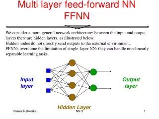
Multi layer feed-forward NN FFNN. We consider a more general network architecture: between the input and output layers there are hidden layers, as illustrated below. Hidden nodes do not directly send outputs to the external environment.

Multi layer feed-forward NN FFNN
E N D
Presentation Transcript
Multi layer feed-forward NNFFNN We consider a more general network architecture: between the input and output layers there are hidden layers, as illustrated below. Hidden nodes do not directly send outputs to the external environment. FFNNs overcome the limitation of single-layer NN: they can handle non-linearly separable learning tasks. Input layer Output layer Hidden Layer NN 3
XOR problem A typical example of a non-linealy separable function is the XOR. This function takes two input arguments with values in {-1,1} and returns one output in {-1,1}, as specified by the following table: If we think at -1 and 1 as encoding of the truth values false and true, respectively, then XOR computes the logical exclusive or, which yields true if and only if the two inputs have different truth values. NN 3
x2 1 -1 1 x1 -1 XOR problem In this graph of the XOR, input pairs giving output equal to 1 and -1 are depicted with green and red circles, respectively. These two classes (green and red) cannot be separated using one line, but two lines. The NN below with two hidden nodes realizes this non-linear separation, where each hidden node represents one of the two blue lines. This specific NN uses the sign activation function. Each green arrow is characterized by the weights of one hidden node. It indicates the direction orthogonal to the corresponding line. It points to the region where the neuron output is 1. The output node is used to combine the outputs of the two hidden nodes. -1 0.1 x1 +1 +1 -1 x2 -1 +1 +1 NN 3 -1
1 w0 x1 w1 x2 w2 1 L1 1 L2 1 Convex region x1 1 L4 L3 1 x2 1 1 1 x1 1 1 x2 1 Types of decision regions Network with a single node One-hidden layer network that realizes the convex region: each hidden node realizes one of the lines bounding the convex region -3.5 P1 two-hidden layer network that realizes the union of three convex regions: each box represents a one hidden layer network realizing one convex region P2 P3 1.5 NN 3
A B B A B A A B B A B A A B B A B A Different Non-LinearlySeparable Problems Types of Decision Regions Exclusive-OR Problem Classes with Meshed regions Most General Region Shapes Structure Single-Layer Half Plane Bounded By Hyperplane Two-Layer Convex Open Or Closed Regions Arbitrary (Complexity Limited by No. of Nodes) Three-Layer NN 3
1 Increasing a -10 -8 -6 -4 -2 2 4 6 8 10 FFNN NEURON MODEL • The classical learning algorithm of FFNN is based on the gradient descent method. For this reason the activation function used in FFNN are continuous functions of the weights, differentiable everywhere. • A typical activation function that can be viewed as a continuous approximation of the step (threshold) function is the Sigmoid Function. A sigmoid function for node j is: • when a tends to infinity then tends to the step function NN 3
Training: Backprop algorithm • The Backprop algorithm searches for weight values that minimize the total error of the network over the set of training examples (training set). • Backprop consists of the repeated application of the following two passes: • Forward pass: in this step the network is activated on one example and the error of (each neuron of) the output layer is computed. • Backward pass:in this step the network error is used for updating the weights (credit assignment problem). This process is more complex than the LMS algorithm for Adaline, because hidden nodes are linked to the error not directly but by means of the nodes of the next layer.Therefore,starting at the output layer, the error is propagated backwards through the network, layer by layer. This is done by recursively computing the local gradient of each neuron. NN 3
Backprop • Back-propagation training algorithm illustrated: • Backprop adjusts the weights of the NN in order to minimize the network total mean squared error. Network activation Error computation Forward Step Error propagation Backward Step NN 3
Total Mean Squared Error • The error of output neuron j after the activation of the network on the n-th training example is: • The network error is the sum of the squared errors of the output neurons: • The total mean squared error is the average of the network errors over the training examples. NN 3
Weight Update Rule The Backprop weight update rule is based on the gradient descent method: take a step in the direction yielding the maximum decrease of the network error E. This direction is the opposite of the gradient of E. NN 3
Error backpropagation The flow-graph below illustrates how errors are back-propagated to the hidden neuron j w1j e1 ’(v1) 1 j ’(vj) wkj ek ’(vk) k wm j em m ’(vm) NN 3
Summary: Delta Rule • Delta rulewji = j yi IF j output node IF j hidden node where for sigmoid activation functions NN 3
Dynamics of BP learning FNN have complex error surfaces (e.g. plateaus, long valleys etc. ) with no single minimum For complex error surfaces the problem is learning rate must keep small to prevent divergence. Adding momentum term is a simple approach dealing with this problem. NN 3
Generalized delta rule • If is smallthen the algorithm learns the weights very slowly, while if is large then the large changes of the weights may cause an unstable behavior with oscillations of the weight values. • A technique for tackling this problem is the introduction of a momentum term in the delta rule which takes into account previous updates. We obtain the following generalized Delta rule: momentum constant momentum term accelerates the descent in steady downhill directions and has a stabilizing effect in directions that oscillate in time. NN 3
Other techniques: adaptation Other heuristics for accelerating the convergence of the back-prop algorithm through adaptation: • Heuristic 1: Every weight has its own . • Heuristic 2: Every is allowed to vary from one iteration to the next. NN 3
Network training: • Two types of network training: • Incremental mode (on-line, stochastic, or per-pattern) • Weights updated after each pattern is presented • Batch mode (off-line or per -epoch) Weights updated after all the patterns are presented NN 3
Backprop algorithmincremental-mode n=1; initializew(n) randomly; while (stopping criterion not satisfied and n<max_iterations) for each example (x,d) - run the network with input x and compute the output y - update the weights in backward order starting from those of the output layer: with computed using the (generalized) Delta rule end-for n = n+1; end-while; choose a randomized ordering for selecting the examples in the training set in order to avoid poor performance. NN 3
Backprop algorithmbatch mode • In the batch-mode the weights are updated only after all examples have been processed, using the formula • The learning process continues on an epoch-by-epoch basis until the stopping condition is satisfied. NN 3
Advantages and disadvantages of different modes • Sequential mode: • Less storage for each weighted connection • Random order of presentation and updating per pattern means search of weight space is stochastic--reducing risk of local minima able to take advantage of any redundancy in training set (i.e.. same pattern occurs more than once in training set, esp. for large training sets) • Simpler to implement • Batch mode: • Faster learning than sequential mode NN 3
Stopping criterions • Sensible stopping criterions: • total mean squared error change: Back-prop is considered to have converged when the absolute rate of change in the average squared error per epoch is sufficiently small (in the range [0.01, 0.1]). • generalization based criterion: After each epoch the NN is tested for generalization using a different set of examples (validation set). If the generalization performance is adequate then stop. NN 3
Use of Available Data Set for Training The available data set is normally split into three sets as follows: • Training set – use to update the weights. Patterns in this set are repeatedly in random order. The weight update equation are applied after a certain number of patterns. • Validation set – use to decide when to stop training only by monitoring the error. • Test set – Use to test the performance of the neural network. It should not be used as part of the neural network development cycle. NN 3
Earlier Stopping - Good Generalization • Running too many epochs may overtrain the network and result in overfitting and perform poorly in generalization. • Keep a hold-out validation set and test accuracy after every epoch. Maintain weights for best performing network on the validation set and stop training when error increases increases beyond this. Validation set error Training set No. of epochs NN 3
Model Selection by Cross-validation • Too few hidden units prevent the network from learning adequately fitting the data and learning the concept. • Too many hidden units leads to overfitting. • Similar cross-validation methods can be used to determine an appropriate number of hidden units by using the optimal test error to select the model with optimal number of hidden layers and nodes. Validation set error Training set No. of epochs NN 3
NN DESIGN • Data representation • Network Topology • Network Parameters • Training • Validation NN 3
Data Representation • Data representation depends on the problem. In general NNs work on continuous (real valued) attributes. Therefore symbolic attributes are encoded into continuous ones. • Attributes of different types may have different ranges of values which affect the training process. Normalization may be used, like the following one which scales each attribute to assume values between 0 and 1. for each value of attribute , where are the minimum and maximum value of that attribute over the training set. NN 3
Network Topology • The number of layers and of neurons depend on the specific task. In practice this issue is solved by trial and error. • Two types of adaptive algorithms can be used: • start from a large network and successively remove some neurons and links until network performance degrades. • begin with a small network and introduce new neurons until performance is satisfactory. NN 3
Network parameters • How are the weights initialized? • How is the learning rate chosen? • How many hidden layers and how many neurons? • How many examples in the training set? NN 3
Initialization of weights • In general, initial weights are randomly chosen, with typical values between -1.0 and 1.0 or -0.5 and 0.5. • If some inputs are much larger than others, random initialization may bias the network to give much more importance to larger inputs. In such a case, weights can be initialized as follows: For weights from the input to the first layer For weights from the first to the second layer NN 3
Choice of learning rate • The right value of depends on the application. Values between 0.1 and 0.9 have been used in many applications. • Other heuristicsadapt during the training as described in previous slides. NN 3
Size of Training set • Rule of thumb: • the number of training examples should be at least five to ten times the number of weights of the network. • Other rule: |W|= number of weights a=expected accuracy NN 3
Expressive Power of FFNN Boolean functions: • Every boolean function can be described by a network with a single hidden layer • but it might require exponential (in the number of inputs) hidden neurons. Continuous functions: • Every bounded piece-wise continuous function can be approximated with arbitrarily small error by a network with one hidden layer. • Any continuous function can be approximated to arbitrary accuracy by a network with two hidden layers. NN 3
Applications of FFNN Classification, pattern recognition: • FFNN can be applied to tackle non-linearly separable learning tasks. • Recognizing printed or handwritten characters • Face recognition • Classification of loan applications into credit-worthy and non-credit-worthy groups • Analysis of sonar radar to determine the nature of the source of a signal Regression and forecasting: • FFNN can be applied to learn non-linear functions (regression) and in particular functions whose inputs is a sequence of measurements over time (time series). NN 3
Engine management • The behaviour of a car engine is influenced by a large number of parameters • temperature at various points • fuel/air mixture • lubricant viscosity. • Major companies have used neural networks to dynamically tune an engine depending on current settings. NN 3
Feed forward NN • Idea: Credit assignment problem • Problem of assigning ‘credit’ or ‘blame’ to individual elements involving in forming overall response of a learning system (hidden units) • In neural networks, problem relates to distributing the network error to the weights. NN 3
ALVINN Drives 70 mph on a public highway 30 outputs for steering 30x32 weights into one out of four hidden unit 4 hidden units 30x32 pixels as inputs NN 3
Application: NETtalk (Sejnowski & Rosenberg, 1987) • The task is to learn to pronounce Englishtext from examples (text-to-speech). • Training data is 1024 words from a side-by-side English/phoneme source. • Input: 7 consecutive characters from written text presented in a moving window that scans text • Output: phoneme code giving the pronunciation of the letter at the center of the input window • Network topology: 7x29 binary inputs (26 chars + punctuation marks), 80 hidden units and 26 output units (phoneme code). Sigmoid units in hidden and output layer. NN 3
NETtalk (contd.) • Training protocol: 95% accuracy on training set after 50 epochs of training by full gradient descent. 78% accuracy on a set-aside test set. • Comparison against Dectalk (a rule based expert system): Dectalk performs better; it represents a decade of analysis by linguists. NETtalk learns from examples alone and was constructed with little knowledge of the task. NN 3
Signature recognition • Each person's signature is different. • There are structural similarities which are difficult to quantify. • One company has manufactured a machine which recognizes signatures to within a high level of accuracy. • Considers speed in addition to gross shape. • Makes forgery even more difficult. NN 3
Sonar target recognition • Distinguish mines from rocks on sea-bed • The neural network is provided with a large number of parameters which are extracted from the sonar signal. • The training set consists of sets of signals from rocks and mines. NN 3
Stock market prediction • “Technical trading” refers to trading based solely on known statistical parameters; e.g. previous price • Neural networks have been used to attempt to predict changes in prices. • Difficult to assess success since companies using these techniques are reluctant to disclose information. NN 3
Mortgage assessment • Assess risk of lending to an individual. • Difficult to decide on marginal cases. • Neural networks have been trained to make decisions, based upon the opinions of expert underwriters. • Neural network produced a 12% reduction in delinquencies compared with human experts. NN 3
1 w0 w1 x1 w2 x2 Questions for the preparation of the final exam • Describe the architecture, neuron model and learning algorithm of the perceptron. • Describe the architecture, neuron model and learning algorithm of the adaline. • What are the conditions under which the perceptron algorithm is ensured to terminate successfully? • Explain the differences between adaline and perceptron. • What are the limitations of single-layer neural networks? • Give an example of a learning problem that cannot be solved using a single-layer neural network. • Derive the Delta rule for the following network: NN 3
Questions for the preparation of the final exam w1 x1 u1 w2 v1 • Derive the Delta rule for the following network • Show that every boolean function can be computed by a FFNN with one hidden layer. • Describe the types of decision regions that can be specified using the following NN architectures: • single layer NN • FFNN with one hidden node • FFNN with two hidden nodes • Describe the FFNN neuron model and explain why the step function cannot be used as activation function in the backprop learning algorithm. • Describe the backprop algorithm. x2 u2 v2 NN 3