15. Query Optimization
15. Query Optimization. System Design Parsing Examples Modern Optimizers EXPLAIN – the output of an optimizer Overview of internals Dynamic programming VP – view the internals Examples Variants Top Down Optimization Optimizer Hints Unnesting Queries. Learning Objectives.

15. Query Optimization
E N D
Presentation Transcript
15. Query Optimization • System Design • Parsing • Examples • Modern Optimizers • EXPLAIN – the output of an optimizer • Overview of internals • Dynamic programming • VP – view the internals • Examples • Variants • Top Down Optimization • Optimizer Hints • Unnesting Queries
Learning Objectives • Explain EXPLAIN • Explain VP’s output • Explain each variant • Flatten a nested query.
Web Form Applic. Front end SQL interface Overview of Query Processing SQL Security Parser Catalog Relational Algebra(RA) Optimizer Executable Plan (RA+Algorithms) Concurrency Plan Executor Files, Indexes & Access Methods Crash Recovery Database, Indexes
Now we focus on the top of this diagram Relation Algebra Query SQL Query Parser Query Optimizer Relational Operator Algs. Files and Access Methods Buffer Management Disk Space Management DB
Detail of the top Query Parser SQL Query(SELECT …) Relational Algebra Expression (Query Tree) Query Optimizer Plan Generator Plan Cost Estimator Catalog Manager Query Tree + Algorithms (Plan) Plan Evaluator
Parsing and Optimization • The Parser • Verifies that the SQL query is syntactically correct, that the tables and attributes exist, and that the user has the appropriate permissions. • Translates the SQL query into a simple query tree(operators: relational algebra plus a few other ones) • The Optimizer: • Generates other, equivalent query trees(Actually builds these trees bottom up) • For each query tree generated: • Selects algorithms for each operator (producing a query plan) • estimates the cost of the plan • Chooses the plan with lowest cost (of the plans considered, which is not necessarily all possible plans)
Schema for Examples • Download Postgres source from • postgresql.org/download • Logical and physical schema is at • src/test/bench/create.source • Simplified version is at • www.cs.pdx.edu/587/create.bench • Log into the database at • https://www.cat.pdx.edu/pgCS587/ • Click on PostgreSQL • User CS587, Password 587dbms, see notes view • Browse the tables, especially tenk1 and its attributes unique1, unique2, stringu1
Here’s what the parser does SQL Query: Relational Algebra Tree: SELECT tenk1.unique1 FROM tenk1 JOIN tenk2 USING unique2 WHERE tenk1.stringu1='xxx'; tenk1.unique1 tenk1.stringu1='xxx' ⋈ Unique2=unique2 tenk2 tenk1
Practice: Parse a Query • Describe the parser's output when the input is SELECT stringu2 FROM tenk1 JOIN tenk2 USING unique1 WHERE tenk1.stringu1='abc';
How Can We View the Optimizer? • Postgres calls its optimizer the Planner • Postgres' planner algorithm [668] is the same as all modern DBMSs' optimizer algorithms • Except SQL Server • We have good news and good news. • We can see both the planner's output AND its internal processing. • Its output is available to anyone; its internal processing is avaliable only to us and a few others. • The output is displayed by the EXPLAIN statement • Every DBMS has a version of EXPLAIN (e.g., SHOW PLAN)
Postgres’ EXPLAIN • Output for EXPLAIN SELECT * FROM tenk1; Seq Scan on tenk1 (cost=0.00.. 445.00 rows=10000 width=244) • These values are estimates from sampling. • Very useful when a query runs longer than expected. • All our examples are from • www.postgresql.org/docs/8.3/interactive/using-explain.html *Actually this includes CPU costs but we will call it I/O costs to simplify Sequential Scan I/Os to get first row* I/Os to get last row* Rows retrieved Average Row Width
More EXPLAIN examples • EXPLAIN SELECT * FROM tenk1 WHERE unique1 < 7000; • Seq Scan on tenk1 (cost=0.00..470.00 rows=7124 width=244) • Filter: (unique1 < 7000) • Cost is higher because of CPU cost for filtering • #rows is off because of estimation using histogram • EXPLAIN SELECT * FROM tenk1 WHERE unique1 < 1; • Index Scan using tenk1_unique1 on tenk1 (cost=0.00..8.27 rows=1 width=244) • Index Cond: (unique1 < 1) • Why is the cost so much less? • EXPLAIN SELECT * FROM tenk1 WHERE unique1 < 10; • Bitmap Heap Scan on tenk1 (cost=4.34..42.58 rows=11 width=244) • Recheck Cond: (unique1 < 10) • -> Bitmap Index Scan on tenk1_unique1 (cost=0.00..4.33 rows=11 width=0) • Index Cond: (unique1 < 10) • Shopping list optimization!
The planner's internal processing • So far we've seen the planner's output: its opinion as to what is the fastest plan. How does it reach that conclusion? • Fortunately, our TA, Tom Raney, has just added a patch to PostgreSQL (PG) that allows anyone to look inside the planner. • This was part of a Google Summer of Code project • One of the lead PG developers says “it’s like finding Sasquatch”. • No other DBMS has this capability. • We’ll use Tom’s patch to view the planner's internals.
Overview of DBMS Optimizers • Recall that "optimizing a query" consists of these 4 tasks • Generate all trees equivalent to the parser-generated tree* • Assign algorithms to each node of each tree • A tree with algorithms is called a plan**. • Calculate the cost of each generated plan • Using the join cost formulas we learned in previous slides*** • Choose the cheapest plan *A nice independent study project would be to write a visualizer for the parser **Use Raney's Visual Planner here to look at a plan *** Statistics for calculating these costs are kept in the systemcatalog.
Dynamic Programming • A no-brainer approach to these 4 tasks could take forever. For medium-large queries there are millions of plans and it can take a millisecond to compute each plan cost, resulting in hours to optimize a query. • This problem was solved in 1979 [668] by Patsy Selinger's IBM team using Dynamic Programming. • The trick is to solve the problem bottom-up: • First optimize all one-table subqueries • Then use those optimal plans to optimize all two-table subqueries • Use those results to optimize all three-table subqueries, etc.
Consider A Query and its Parsed Form SELECT tenk1.unique1 FROM tenk1 JOIN tenk2 USING (unique2) WHERE tenk1.unique1< 100; tenk1.unique1 tenk1.unique1<100 ⋈ unique2=unique2 tenk2 tenk1
What Will a Selinger-type Optimizer Do? • Optimize one table subqueries • tenk1 WHERE unique1<100 • This is called "pushing selects" • Then optimize tenk2 • Use the results of the previous steps to Optimize two-table queries • The entire query • Let's use Raney's patch, the Visual Planner, to see what PG's Planner does.
How to Set Up Your Visual Planner • Download, then unzip, in Windows or *NIX: • cs.pdx.edu/~len/587/VP1.7.zip • Read README.TXT, don't worry about details • Be sure your machine has a Java VM • http://www.java.com/en/download/index.jsp • Click on Visual_Planner.jar • If that does not work, use this at the command line: • java -jar Visual_Planner.jar • In the resulting window • File/Open • Navigate to the directory where you put VP1.7 • Navigating to C: may take a while • Choose plan1.pln
Windows in the Visual Planner • The SQL window holds the (canned) query • The Plan Tree window holds the optimal plan for the query (in this VP view). • The Statistics window holds statistics about the highlighted node of the Plan Tree's plan • Click a Plan Treenode to see its statistics • Why is a nested loop the optimal plan?
Why Not? • To see other plans, click on tenk1/tenk2 in the ROI window. • Then shift-click the plan you want to see • Plans are in alphabetical order, then by total cost • Why isn't a merge join cheaper? • Why isn't a hash join cheaper?
Visualize Dynamic Programming • Recall the first steps of Dynamic Programming: • Optimize tenk1 where unique1<100 • Optimize tenk2. • VP calls these the ROI* steps and they are displayed in the ROI window of VP. • In the ROI window, click on the symbol next to tenk2 to see how the PG Planner optimized tenk2. • Note that blue plans are saved for later steps, red plans are discarded. *Postgres uses an internal data structure called RelOptInfo to hold the relations currently being optimized
Optimizing tenk2; Interesting Orders • The cheapest access path(plan)* is a sequential scan. • However, an index scan is also saved. Why? Because the index scan has an order associated with it, and the order is an interesting order. • The order is unique2, and unique2 is the joining attribute for the later join. • It may be worth sacrificing some cost here to save the cost of a sort later! *plan = access path since tenk2 is a single table
Optimizing tenk1 • Explain each of the planner's decisions in its optimization of tenk1.
Variants on what we've discussed • SQLServer: Top down • Graefe, McKenna, “The Cascades Framework for query optimization”, DEBulletin, 1995. • Hints • Rewrite optimization rules: unnesting
Top Down Optimization • Begin with original query • Consider subqueries, optimize them. • Depth first search • Example: A ⋈ B ⋈ C • First optimize, say, (A ⋈ B) ⋈C. • If its cost is less than B ⋈ C, need not calculate the cost of A ⋈ (B ⋈C). • Memo structure used to keep track of optimized subqueries.
Optimizer Hints • A hint tells the optimizer to ignore its algorithm in part, for example • Order the joins in a certain way • Use a particular index • Use a type of join for a pair of tables. • Oracle has over 120 possible hints • www.dba-oracle.com/art_otn_cbo_p7.htm • SQL Server • www.sql-server-performance.com/tips/hints_general_p1.aspx
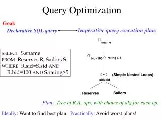
15.5 Nested Queries SELECT S.sid FROM Sailors S WHERE EXISTS (SELECT * FROM Reserves R WHERE R.bid=103 AND R.sid=S.sid) • No-brainer method for executing nested queries • Tuple iteration semantics • For each outer tuple, evaluate inner block • Equivalent to simple nested loop join • Optimizer optimizes inner block, then outer block • Is there a better way? Nested block to optimize: SELECT * FROM Reserves R WHERE R.bid=103 AND R.sid= outer value
Unnesting queries Equivalent non-nested query: SELECT DISTINCT S.sid FROM Sailors S, Reserves R WHERE S.sid=R.sid AND R.bid=103 • Optimizer (proprietary systems mostly) or you (open source systems mostly) unnest nested queries. • If the query is unnested, the optimizer can use bulk join algorithms (merge, hash join) and performance can be much better.
Unnesting with COUNT SELECT S.sname FROM Sailors S WHERE S.rank > (SELECT COUNT(R.*) FROM Reserves R WHERER.sid=S.sid) • Beware if there is a COUNT in the subquery • The query may appear to unnest into a join with a GROUP BY. • But consider a sailor with a high rank and no reservations SELECT S.sname FROM Sailors S, Reserves R WHERE S.sid=R.sid GROUP BY S.sid HAVING S.rank > COUNT(R.*)
Unnesting – The Count Bug [298] SELECT S.sname FROM Sailors S WHERE S.rank > (SELECT * FROM Reserves R WHERE R.sid=S.sid) • The query may not unnest into a join, but rather an outer join. • Many queries are much harder or impossible to unnest! SELECT S.sname FROM Sailors S NATURAL RIGHT OUTER JOIN Reserves R GROUP BY S.sid HAVING S.rank > COUNT(R.*)

