Understanding Time Complexity: P Class, Big-O Notation, and Turing Machines
This agenda explores crucial concepts in computational theory, focusing on time complexity classes, particularly the class P, and the relationship between Turing machines (TMs) and RAM programs. It covers Big-O notation, decision problem encodings, polynomial and exponential time complexities, and the implications of the Strong Church-Turing thesis. The course aims to clarify the differences in performance between polynomial-time algorithms and those requiring exponential time, alongside exploring the challenge of factoring numbers and context-free languages.


Understanding Time Complexity: P Class, Big-O Notation, and Turing Machines
E N D
Presentation Transcript
The class P Zeph Grunschlag
Agenda • Running time • Big-O review • Time complexity classes • The class P • Converting RAM programs to TM programs with polynomial loss of efficiency • Decision problems encoding I/O problems • Factoring numbers • Context free languages are in P • CYK algorithm
Polynomial Time vs.Exponential Time Experience shows that the dividing line between problems solvable in polynomial time vs. those requiring exponential time is fundamental. Let’s define the running time of TM’s: DEF: The running time of a Turing machine M is the function f (n) which is the maximum number of transitions that M takes to halt when given an arbitrary input of length n. NOTE: A crash is considered as halting.
Running Time 0R acc rej Q: What the running time of the above? 0 R 0R 1R 2 1 1R 0R 1R
Running Time 0R acc rej A: Assuming S = {0,1}, the running time is T (n)=n+1` as can be seen on any input starting with 1. Even though the TM runs faster on 0{0,1}*, running time is defined in terms of the worst case. Crashes don’t affect this. 0 R 0R 1R 2 1 1R 0R 1R
Polynomial Time Complexity DEF: M is of polynomial time complexity if there is a polynomial p(n) for with the running time f (n) of M satisfies: f (n) p(n) . Problem: Nobody uses Turing machines in the real world so is this really justified. Resolution: Investigate the efficiency of Turing machines vs. actual RAM machines: Strong Church-Turing Thesis: Any computing device can be simulated by TM’s with at worst a polynomial time slow-down.
Strong Church-Turing Thesis? As opposed to the standard Church-Turing thesis for which there is overwhelming evidence, there is a great deal of current research trying to show that the strong version is false. In particular: Possible Counterexample: Many conjecture that no polynomial time algorithm exists for factoring numbers using a TM. But a polynomial time quantum algorithm exists (Peter Shor). Would mean that quantum computers invalidate Strong C-T thesis!
Big-O Notation Nothing to say here. Assume you learned in Discrete Math and Data Structures.
Big-O Notation OK… here’s a refresher: DEF: Let f and g be functions with domain R0 or N and codomain R. If there are constants C and k such x > k,|f (x )| C |g (x )| i.e., past k,f is less than or equal to a multiple of g, then we write: f (x ) = O ( g (x ) )
Big- and Big- Big- is just the reverse of big-O. I.e. f (x ) = (g (x )) g (x ) = O (f (x )) So big- says that asymptotically f (x ) dominatesg (x ). Big- says that both functions dominate each-other so are asymptotically equivalent. I.e. f (x ) = (g (x )) f (x ) = O (g (x )) f (x ) = (g (x )) Synonym for f = (g): “f is of orderg ”
Useful facts • Any polynomial is big- of its largest term • EG: x 4/100000 + 3x 3 + 5x 2 – 9 =(x 4) • The sum of two functions is big-O of the biggest • EG: x 4 ln(x ) + x 5 = O (x 5) • Non-zero constants are irrelevent: • EG: 17x 4 ln(x ) = O (x 4 ln(x ))
Big-O, Big-, Big-. Examples Q: Order the following from smallest to largest asymptotically. Group together all functions which are big- of each other:
Big-O, Big-, Big-. Examples A: 1. 2. 3. , (change of base formula) 4. 5. 6. 7. 8. 9. 10.
Time Complexity Classes Time complexity classes are the next languages classes that we’ll study: DEF: Suppose that g (n) is a real function. The time complexity class TIME(g (n) ) consists of all languages which are decided by some TM with running time O(g (n)). Any such language is said to by oftime complexity g (n).
Time Complexity 0R acc rej Q: For which g (n) is the language accepted above of time complexity g (n) ? • g (n) = n +2 • g (n) = n/2 • g (n) = n2 • g (n) = 1 0 R 0R 1R 2 1 1R 0R
Time Complexity 0R acc rej A: ALL! This particular decider for the language has running time f (n) = n+2 which is big-O of no.’s 1, 2 and 3. But the definition doesn’t say that must stick to any single implementation: Q: How would you modify the TM to see that accepted language is in TIME(1) ? 0 R 0R 1R 2 1 1R 0R
Time Complexity A: Accepted language is 10{0,1}*. So just need to check first two bits as pictured below: So now we see that the language is accepted by a TM which runs in constant time. R 0R 1R 1R 0R 0 1 2 acc
The Class P P is the class of languages that are decided by a TM of time complexity some polynomial. IE: DEF:
From RAM to TM in Polynomial Time THM 1: Any RAM program which runs in O (f (n)) time can be simulated by a multi-tape TM which runs in O (f (n)3 ) time. THM 2: Any multi-tape TM which runs in O (g (n)) time can be simulated by a one-tape TM which runs in O (g (n)2 ) time. COR: Any RAM program which runs in O (f (n)) time can be simulated by a one-tape TM which runs in O (f (n)6 ) time. Consequently, any algorithm that runs in polynomial time on your desktop, can be made to run in polynomial time on a TM.
From RAM to TM in Polynomial Time No proofs. Rather, give brief explanation: • A RAM consists of a “goto” style program and a memory made up of arbitrarily many integers called registers and each having an integer address. A single step of a RAM consists of doing something to one of the registers1. After k steps, a RAM may have at most O (k)active registers each containing an integer of length O (k). If we keep these contents on one of the TM tapes, changing the state of the simulated RAM requires reading all O (k) registers each of size O (k), so O (k 2) tape cells. Since k = O (f (n) ), and there are f (n) steps to simulate, g(n) = O (f (n)3 ).
From RAM to TM in Polynomial Time • On the other hand, recall conversion from a multi-tape to a 1-tape TM. Converted to a multi-track machine first. The multi-track machine needed to sweep back and forth once across whole tape to read the current active cells. So on multitape’s k ’th step, contents are O (k) so sweeping back and forth is O(k ). Since k = O (g (n) ), and there are g (n) steps to simulate, h(n) = O (g (n)2 ). • Now go from multitrack to one-tape machine. Recall that all we did was rename alphabet and transitions so running time was identical to that of 1-tape simulator and to that of k-tape TM!
RAM’s are Polynomially Equivalent to TM’s Other direction valid as well: Can simulate any TM in the same asymptotic time complexity in Java. Conclude: The belonging of a given language to the class P does not depend on the computing paradigm chosen. Thus pseudocode is useful in analyzing computational complexity.
Turning Decision Problems into I/O Problems Up till now, point of view of course has been to study computability of algorithmic problems by looking at decision problem versions. However, in practice, decision problems aren’t always interesting. EG: If you want to break the RSA encryption algorithm knowing that a number N is composite isn’t good enough. Would want to output the prime factors as well!
Encoding FACTORING by a Decision Problem It turns out, that usually I/0 problems can easily be encoded as decision problems which can yield solutions to the original I/O problem with only polynomial loss of efficiency. EG: Consider I/O problem FACTORING: Input: a number n Output: a set of prime numbers p1,p2,…,pt whose product is the number n.
Encoding FACTORING by a Decision Problem Encode FACTORING by the decision problem BOUNDED_FACTOR: Given: a number pair (n,k) Decide: is there a number d strictly between 1 and k which divides n ? Q: Which of the following are in BOUNDED_FACTOR: • (10,5) • (7,8) • (7,7)
Encoding FACTORING by a Decision Problem A: Which of the following are in BOUNDED_FACTOR: • (10,5) Yes, because 2 divides 10 and 1<2<5. • (7,8) Yes, because 7 divides itself and 1<7<8 • (7,7) No, because 7 is prime so does not contain any factors between 1 & 7. Q: How can PRIME be reduced to BOUNDED_FACTOR ?
Encoding FACTORING by a Decision Problem A: Use the co-mapping reduction f : PRIME BOUNDED_FACTOR defined by f (n) = (n,n). Now let’s see how to turn a solution to BOUNDED_FACTOR into a factoring algorithm with polynomial loss of efficiency. The idea is to use a binary search to look for a prime factor. Then divide out by the factor and repeat:
Encoding FACTORING by a Decision Problem m = n, i = 0 while(m > 1) i = i + 1 k = 0, l = m + 1 while( k < l - 1 ) if( BOUNDED_FACTOR(m,(k+l)/2) ) l = (k+l)/2 else k = (k+l)/2 pi = k // the smallest prime factor of m m = m/k return (p1, p2 , … , pi)
m = n, i = 0 while(m > 1) i = i+1 k = 0, l = m+1 while( k < l-1 ) if(BOUNDED_FACTOR(m,(k+l)/2)) l = (k+l)/2 else k = (k+l)/2 pi=k //smallest prime factor ofm m = m/k return (p1, p2 , … , pi) Let’s see how the algorithm works on input n = 12 Encoding FACTORING by a Decision Problem
m = n, i = 0 while(m > 1) i = i+1 k = 0, l = m+1 while( k < l-1 ) if(BOUNDED_FACTOR(m,(k+l)/2)) l = (k+l)/2 else k = (k+l)/2 pi=k //smallest prime factor ofm m = m/k return (p1, p2 , … , pi) Prime factors: Encoding FACTORING by a Decision Problem EG n=12
m = n, i = 0 while(m > 1) i = i+1 k = 0, l = m+1 while( k < l-1 ) if(BOUNDED_FACTOR(m,(k+l)/2)) l = (k+l)/2 else k = (k+l)/2 pi=k //smallest prime factor ofm m = m/k return (p1, p2 , … , pi) Prime factors: Encoding FACTORING by a Decision Problem EG n=12
m = n, i = 0 while(m > 1) i = i+1 k = 0, l = m+1 while( k < l-1 ) if(BOUNDED_FACTOR(m,(k+l)/2)) l = (k+l)/2 else k = (k+l)/2 pi=k //smallest prime factor ofm m = m/k return (p1, p2 , … , pi) Prime factors: Encoding FACTORING by a Decision Problem EG n=12
m = n, i = 0 while(m > 1) i = i+1 k = 0, l = m+1 while( k < l-1 ) if(BOUNDED_FACTOR(m,(k+l)/2)) l = (k+l)/2 else k = (k+l)/2 pi=k //smallest prime factor ofm m = m/k return (p1, p2 , … , pi) Prime factors: Encoding FACTORING by a Decision Problem EG n=12
m = n, i = 0 while(m > 1) i = i+1 k = 0, l = m+1 while( k < l-1 ) if(BOUNDED_FACTOR(m,(k+l)/2)) l = (k+l)/2 else k = (k+l)/2 pi=k //smallest prime factor ofm m = m/k return (p1, p2 , … , pi) Prime factors: Encoding FACTORING by a Decision Problem EG n=12
m = n, i = 0 while(m > 1) i = i+1 k = 0, l = m+1 while( k < l-1 ) if(BOUNDED_FACTOR(m,(k+l)/2)) l = (k+l)/2 else k = (k+l)/2 pi=k //smallest prime factor ofm m = m/k return (p1, p2 , … , pi) Prime factors: Encoding FACTORING by a Decision Problem EG n=12
m = n, i = 0 while(m > 1) i = i+1 k = 0, l = m+1 while( k < l-1 ) if(BOUNDED_FACTOR(m,(k+l)/2)) l = (k+l)/2 else k = (k+l)/2 pi=k //smallest prime factor ofm m = m/k return (p1, p2 , … , pi) Prime factors: Encoding FACTORING by a Decision Problem EG n=12
m = n, i = 0 while(m > 1) i = i+1 k = 0, l = m+1 while( k < l-1 ) if(BOUNDED_FACTOR(m,(k+l)/2)) l = (k+l)/2 else k = (k+l)/2 pi=k //smallest prime factor ofm m = m/k return (p1, p2 , … , pi) Prime factors: Encoding FACTORING by a Decision Problem EG n=12
m = n, i = 0 while(m > 1) i = i+1 k = 0, l = m+1 while( k < l-1 ) if(BOUNDED_FACTOR(m,(k+l)/2)) l = (k+l)/2 else k = (k+l)/2 pi=k //smallest prime factor ofm m = m/k return (p1, p2 , … , pi) Prime factors: 2 Encoding FACTORING by a Decision Problem EG n=12
m = n, i = 0 while(m > 1) i = i+1 k = 0, l = m+1 while( k < l-1 ) if(BOUNDED_FACTOR(m,(k+l)/2)) l = (k+l)/2 else k = (k+l)/2 pi=k //smallest prime factor ofm m = m/k return (p1, p2 , … , pi) Prime factors: 2 Encoding FACTORING by a Decision Problem EG n=12
m = n, i = 0 while(m > 1) i = i+1 k = 0, l = m+1 while( k < l-1 ) if(BOUNDED_FACTOR(m,(k+l)/2)) l = (k+l)/2 else k = (k+l)/2 pi=k //smallest prime factor ofm m = m/k return (p1, p2 , … , pi) Prime factors: 2 Encoding FACTORING by a Decision Problem EG n=12
m = n, i = 0 while(m > 1) i = i+1 k = 0, l = m+1 while( k < l-1 ) if(BOUNDED_FACTOR(m,(k+l)/2)) l = (k+l)/2 else k = (k+l)/2 pi=k //smallest prime factor ofm m = m/k return (p1, p2 , … , pi) Prime factors: 2 Encoding FACTORING by a Decision Problem EG n=12
m = n, i = 0 while(m > 1) i = i+1 k = 0, l = m+1 while( k < l-1 ) if(BOUNDED_FACTOR(m,(k+l)/2)) l = (k+l)/2 else k = (k+l)/2 pi=k //smallest prime factor ofm m = m/k return (p1, p2 , … , pi) Prime factors: 2 Encoding FACTORING by a Decision Problem EG n=12
m = n, i = 0 while(m > 1) i = i+1 k = 0, l = m+1 while( k < l-1 ) if(BOUNDED_FACTOR(m,(k+l)/2)) l = (k+l)/2 else k = (k+l)/2 pi=k //smallest prime factor ofm m = m/k return (p1, p2 , … , pi) Prime factors: 2 Encoding FACTORING by a Decision Problem EG n=12
m = n, i = 0 while(m > 1) i = i+1 k = 0, l = m+1 while( k < l-1 ) if(BOUNDED_FACTOR(m,(k+l)/2)) l = (k+l)/2 else k = (k+l)/2 pi=k //smallest prime factor ofm m = m/k return (p1, p2 , … , pi) Prime factors: 2 Encoding FACTORING by a Decision Problem EG n=12
m = n, i = 0 while(m > 1) i = i+1 k = 0, l = m+1 while( k < l-1 ) if(BOUNDED_FACTOR(m,(k+l)/2)) l = (k+l)/2 else k = (k+l)/2 pi=k //smallest prime factor ofm m = m/k return (p1, p2 , … , pi) Prime factors: 2, 2 Encoding FACTORING by a Decision Problem EG n=12
m = n, i = 0 while(m > 1) i = i+1 k = 0, l = m+1 while( k < l-1 ) if(BOUNDED_FACTOR(m,(k+l)/2)) l = (k+l)/2 else k = (k+l)/2 pi=k //smallest prime factor ofm m = m/k return (p1, p2 , … , pi) Prime factors: 2, 2 Encoding FACTORING by a Decision Problem EG n=12
m = n, i = 0 while(m > 1) i = i+1 k = 0, l = m+1 while( k < l-1 ) if(BOUNDED_FACTOR(m,(k+l)/2)) l = (k+l)/2 else k = (k+l)/2 pi=k //smallest prime factor ofm m = m/k return (p1, p2 , … , pi) Prime factors: 2, 2 Encoding FACTORING by a Decision Problem EG n=12
m = n, i = 0 while(m > 1) i = i+1 k = 0, l = m+1 while( k < l-1 ) if(BOUNDED_FACTOR(m,(k+l)/2)) l = (k+l)/2 else k = (k+l)/2 pi=k //smallest prime factor ofm m = m/k return (p1, p2 , … , pi) Prime factors: 2, 2 Encoding FACTORING by a Decision Problem EG n=12
m = n, i = 0 while(m > 1) i = i+1 k = 0, l = m+1 while( k < l-1 ) if(BOUNDED_FACTOR(m,(k+l)/2)) l = (k+l)/2 else k = (k+l)/2 pi=k //smallest prime factor ofm m = m/k return (p1, p2 , … , pi) Prime factors: 2, 2 Encoding FACTORING by a Decision Problem EG n=12
m = n, i = 0 while(m > 1) i = i+1 k = 0, l = m+1 while( k < l-1 ) if(BOUNDED_FACTOR(m,(k+l)/2)) l = (k+l)/2 else k = (k+l)/2 pi=k //smallest prime factor ofm m = m/k return (p1, p2 , … , pi) Prime factors: 2, 2 Encoding FACTORING by a Decision Problem EG n=12