Chapter 13: Open Channel Flow
Chapter 13: Open Channel Flow. Eric G. Paterson Department of Mechanical and Nuclear Engineering The Pennsylvania State University Spring 2005. Note to Instructors.

Chapter 13: Open Channel Flow
E N D
Presentation Transcript
Chapter 13: Open Channel Flow Eric G. Paterson Department of Mechanical and Nuclear Engineering The Pennsylvania State University Spring 2005
Note to Instructors These slides were developed1, during the spring semester 2005, as a teaching aid for the undergraduate Fluid Mechanics course (ME33: Fluid Flow) in the Department of Mechanical and Nuclear Engineering at Penn State University. This course had two sections, one taught by myself and one taught by Prof. John Cimbala. While we gave common homework and exams, we independently developed lecture notes. This was also the first semester that Fluid Mechanics: Fundamentals and Applications was used at PSU. My section had 93 students and was held in a classroom with a computer, projector, and blackboard. While slides have been developed for each chapter of Fluid Mechanics: Fundamentals and Applications, I used a combination of blackboard and electronic presentation. In the student evaluations of my course, there were both positive and negative comments on the use of electronic presentation. Therefore, these slides should only be integrated into your lectures with careful consideration of your teaching style and course objectives. Eric Paterson Penn State, University Park August 2005 1 This Chapter was not covered in our class. These slides have been developed at the request of McGraw-Hill
Objectives • Understand how flow in open channels differs from flow in pipes • Learn the different flow regimes in open channels and their characteristics • Predict if hydraulic jumps are to occur during flow, and calculate the fraction of energy dissipated during hydraulic jumps • Learn how flow rates in open channels are measured using sluice gates and weirs
Classification of Open-Channel Flows • Open-channel flows are characterized by the presence of a liquid-gas interface called the free surface. • Natural flows: rivers, creeks, floods, etc. • Human-made systems: fresh-water aqueducts, irrigation, sewers, drainage ditches, etc.
Classification of Open-Channel Flows • In an open channel, • Velocity is zero on bottom and sides of channel due to no-slip condition • Velocity is maximum at the midplane of the free surface • In most cases, velocity also varies in the streamwise direction • Therefore, the flow is 3D • Nevertheless, 1D approximation is made with good success for many practical problems.
Classification of Open-Channel Flows • Flow in open channels is also classified as being uniform or nonuniform, depending upon the depth y. • Uniform flow (UF) encountered in long straight sections where head loss due to friction is balanced by elevation drop. • Depth in UF is called normal depth yn
Classification of Open-Channel Flows • Obstructions cause the flow depth to vary. • Rapidly varied flow (RVF) occurs over a short distance near the obstacle. • Gradually varied flow (GVF) occurs over larger distances and usually connects UF and RVF.
Classification of Open-Channel Flows • Like pipe flow, OC flow can be laminar, transitional, or turbulent depending upon the value of the Reynolds number • Where • = density, = dynamic viscosity, = kinematic viscosity • V = average velocity • Rh = Hydraulic Radius = Ac/p • Ac = cross-section area • P = wetted perimeter • Note that Hydraulic Diameter was defined in pipe flows as Dh = 4Ac/p = 4Rh (Dh is not 2Rh, BE Careful!)
Classification of Open-Channel Flows • The wetted perimeter does not include the free surface. • Examples of Rh for common geometries shown in Figure at the left.
Froude Number and Wave Speed • OC flow is also classified by the Froude number • Resembles classification of compressible flow with respect to Mach number
Froude Number and Wave Speed • Critical depth yc occurs at Fr = 1 • At low flow velocities (Fr < 1) • Disturbance travels upstream • y > yc • At high flow velocities (Fr > 1) • Disturbance travels downstream • y < yc
Froude Number and Wave Speed • Important parameter in study of OC flow is the wave speedc0, which is the speed at which a surface disturbance travels through the liquid. • Derivation of c0 for shallow-water • Generate wave with plunger • Consider control volume (CV) which moves with wave at c0
Froude Number and Wave Speed • Continuity equation (b = width) • Momentum equation
Froude Number and Wave Speed • Combining the momentum and continuity relations and rearranging gives • For shallow water, where y << y, Wave speed c0 is only a function of depth
Specific Energy • Total mechanical energy of the liquid in a channel in terms of heads z is the elevation head y is the gage pressure head V2/2g is the dynamic head • Taking the datum z=0 as the bottom of the channel, the specific energy Es is
Specific Energy • For a channel with constant width b, • Plot of Es vs. y for constant V and b
Specific Energy • This plot is very useful • Easy to see breakdown of Es into pressure (y) and dynamic (V2/2g) head • Es as y 0 • Es y for large y • Esreaches a minimum called the critical point. • There is a minimum Es required to support the given flow rate. • Noting that Vc = sqrt(gyc) • For a given Es > Es,min, there are two different depths, or alternating depths, which can occur for a fixed value of Es • A small change in Es near the critical point causes a large difference between alternate depths and may cause violent fluctuations in flow level. Operation near this point should be avoided.
Continuity and Energy Equations • 1D steady continuity equation can be expressed as • 1D steady energy equation between two stations • Head loss hL is expressed as in pipe flow, using the friction factor, and either the hydraulic diameter or radius
Continuity and Energy Equations • The change in elevation head can be written in terms of the bed slope • Introducing the friction slope Sf • The energy equation can be written as
Uniform Flow in Channels • Uniform depth occurs when the flow depth (and thus the average flow velocity) remains constant • Common in long straight runs • Flow depth is called normal depth yn • Average flow velocity is called uniform-flow velocity V0
Uniform Flow in Channels • Uniform depth is maintained as long as the slope, cross-section, and surface roughness of the channel remain unchanged. • During uniform flow, the terminal velocity reached, and the head loss equals the elevation drop • We can the solve for velocity (or flow rate) • Where C is the Chezy coefficient. f is the friction factor determined from the Moody chart or the Colebrook equation
Best Hydraulic Cross Sections • Best hydraulic cross section for an open channel is the one with the minimum wetted perimeter for a specified cross section (or maximum hydraulic radius Rh) • Also reflects economy of building structure with smallest perimeter
Best Hydraulic Cross Sections • Example: Rectangular Channel • Cross section area, Ac = yb • Perimeter, p = b + 2y • Solve Acfor b and substitute • Taking derivative with respect to • To find minimum, set derivative to zero Best rectangular channel has a depth 1/2 of the width
Best Hydraulic Cross Sections • Same analysis can be performed for a trapezoidal channel • Similarly, taking the derivative of p with respect to q, shows that the optimum angle is • For this angle, the best flow depth is
Gradually Varied Flow • In GVF, y and V vary slowly, and the free surface is stable • In contrast to uniform flow, Sf S0. Now, flow depth reflects the dynamic balance between gravity, shear force, and inertial effects • To derive how how the depth varies with x, consider the total head
Gradually Varied Flow • Take the derivative of H • Slope dH/dx of the energy line is equal to negative of the friction slope • Bed slope has been defined • Inserting both S0 and Sf gives
Gradually Varied Flow • Introducing continuity equation, which can be written as • Differentiating with respect to x gives • Substitute dV/dx back into equation from previous slide, and using definition of the Froude number gives a relationship for the rate of change of depth
Gradually Varied Flow • This result is important. It permits classification of liquid surface profiles as a function of Fr, S0, Sf, and initial conditions. • Bed slope S0 is classified as • Steep : yn < yc • Critical : yn = yc • Mild : yn > yc • Horizontal : S0 = 0 • Adverse : S0 < 0 • Initial depth is given a number • 1 : y > yn • 2 : yn < y < yc • 3 : y < yc
Gradually Varied Flow • 12 distinct configurations for surface profiles in GVF.
Gradually Varied Flow • Typical OC system involves several sections of different slopes, with transitions • Overall surface profile is made up of individual profiles described on previous slides
Rapidly Varied Flow and Hydraulic Jump • Flow is called rapidly varied flow (RVF) if the flow depth has a large change over a short distance • Sluice gates • Weirs • Waterfalls • Abrupt changes in cross section • Often characterized by significant 3D and transient effects • Backflows • Separations
Rapidly Varied Flow and Hydraulic Jump • Consider the CV surrounding the hydraulic jump • Assumptions • V is constant at sections (1) and (2), and 1 and 2 1 • P = gy • w is negligible relative to the losses that occur during the hydraulic jump • Channel is wide and horizontal • No external body forces other than gravity
Rapidly Varied Flow and Hydraulic Jump • Continuity equation • X momentum equation • Substituting and simplifying Quadratic equation for y2/y1
Rapidly Varied Flow and Hydraulic Jump • Solving the quadratic equation and keeping only the positive root leads to the depth ratio • Energy equation for this section can be written as • Head loss associated with hydraulic jump
Rapidly Varied Flow and Hydraulic Jump • Often, hydraulic jumps are avoided because they dissipate valuable energy • However, in some cases, the energy must be dissipated so that it doesn’t cause damage • A measure of performance of a hydraulic jump is its fraction of energy dissipation, or energy dissipation ratio
Rapidly Varied Flow and Hydraulic Jump • Experimental studies indicate that hydraulic jumps can be classified into 5 categories, depending upon the upstream Fr
Flow Control and Measurement • Flow rate in pipes and ducts is controlled by various kinds of valves • In OC flows, flow rate is controlled by partially blocking the channel. • Weir : liquid flows over device • Underflow gate : liquid flows under device • These devices can be used to control the flow rate, and to measure it.
Flow Control and MeasurementUnderflow Gate • Underflow gates are located at the bottom of a wall, dam, or open channel • Outflow can be either free or drowned • In free outflow, downstream flow is supercritical • In the drowned outflow, the liquid jet undergoes a hydraulic jump. Downstream flow is subcritical. Free outflow Drowned outflow
Flow Control and MeasurementUnderflow Gate Schematic of flow depth-specific energy diagram for flow through underflow gates • Es remains constant for idealized gates with negligible frictional effects • Es decreases for real gates • Downstream is supercritical for free outflow (2b) • Downstream is subcritical for drowned outflow (2c)
Flow Control and MeasurementOverflow Gate • Specific energy over a bump at station 2 Es,2 can be manipulated to give • This equation has 2 positive solutions, which depend upon upstream flow.
Flow Control and MeasurementBroad-Crested Weir • Flow over a sufficiently high obstruction in an open channel is always critical • When placed intentionally in an open channel to measure the flow rate, they are called weirs
Flow Control and MeasurementSharp-Crested V-notch Weirs • Vertical plate placed in a channel that forces the liquid to flow through an opening to measure the flow rate • Upstream flow is subcritical and becomes critical as it approaches the weir • Liquid discharges as a supercritical flow stream that resembles a free jet
Flow Control and MeasurementSharp-Crested V-notch Weirs • Flow rate equations can be derived using energy equation and definition of flow rate, and experimental for determining discharge coefficients • Sharp-crested weir • V-notch weir where Cwd typically ranges between 0.58 and 0.62