Download
1 / 28
290 likes | 499 Vues
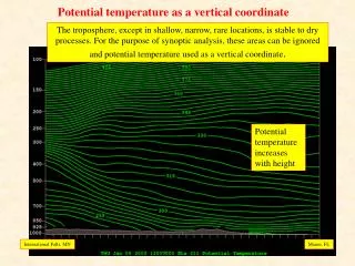
Potential temperature as a vertical coordinate. The troposphere, except in shallow, narrow, rare locations, is stable to dry processes. For the purpose of synoptic analysis, these areas can be ignored and potential temperature used as a vertical coordinate.

E N D
Potential temperature as a vertical coordinate The troposphere, except in shallow, narrow, rare locations, is stable to dry processes. For the purpose of synoptic analysis, these areas can be ignored and potential temperature used as a vertical coordinate. Potential temperature increases with height International Falls, MN Miami, FL
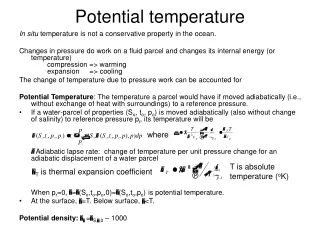
Potential temperature is conserved during an adiabatic process. An adiabatic process is isentropic, that is, a process in which entropy is conserved Entropy = Cp ln(q) + constant = 0 Potential temperature is not conserved when 1) diabatic heating or cooling occurs or 2) mixing of air parcels with different properties occurs Examples of diabatic processes: condensation, evaporation, sensible heating from surface radiative heating, radiative cooling
Isentropic Analyses are done on constant q surfaces, rather than constant P or z Constant pressure surface Constant potential temperature surface
Note that: 1) isentropic surfaces slope downward toward warm air (opposite the slope of pressure surfaces) 2) Isentropes slope much more steeply than pressure surfaces given the same thermal gradient. cold warm
In the absence of diabatic processes and mixing, air flows along q surfaces. Isentropic surfaces act as “material” surfaces, with air parcels thermodynamically bound to the surface unless diabatic heating or cooling occurs. Since isentropic surfaces slope substantially, flow along an isentropic surface contains the adiabatic component of vertical motion.
Vertical motion can be expressed as the time derivative of pressure: WHEN w IS POSITIVE, PRESSURE OF AIR PARCEL IS INCREASING WITH TIME – AIR IS DESCENDING. WHEN w IS NEGATIVE, PRESSURE OF AIR PARCEL IS DECREASING WITH TIME – AIR IS ASCENDING. Let’s expand the derivative in isentropic coordinates: This equation is an expression of vertical motion in an isentropic coordinate system. Let’s look at this equation carefully because it is the key to interpreting isentropic charts
Let’s start with the second term: u v Pressure advection: When the wind is blowing across the isobars on an isentropic chart toward higher pressure, air is descending (w is positive) When the wind is blowing across the isobars on an isentropic chart toward lower pressure, air is ascending (w is negative)
300 K Surface 14 Feb 92 Pressure in mb Wind blowing from low pressure to high pressure- air descending Wind blowing from high pressure to low pressure- air ascending 25 m/s
Interpretation of “Pressure Advection” From the equation for q: On a constant q surface, an isobar (line of constant pressure) must also be an isotherm (line of constant temperature) From the equation of state: P = rRT and equation for q: On a constant q surface, an isobar (line of constant pressure) Must also be an isopycnic (line of constant density) Therefore: On a constant theta surface, pressure advection is equivalent to thermal advection If wind blows from high pressure to low pressure (ascent): Warm advection If wind blows from low pressure to high pressure (descent): Cold advection
300 K Surface 14 Feb 92 Pressure in mb 25 m/s Cold advection Warm advection
Let’s now look at the first term contributing to vertical motion: is the local (at one point in x, y) rate of change of pressure of the theta surface with time. is negative since the pressure at a point on the theta surface is decreasing with time. If the theta surface rises, is positive since the pressure at a point on the theta surface is increasing with time. If the theta surface descends,
Position of the 330 K isentrope at 00 UTC on 12 Jan 2003 Position of the 330 K isentrope at 12 UTC on 10 Jan 2003
Vertical displacement of isentrope = (Air must rise for isentrope to be displaced upward)
Let’s now look at the third term contributing to vertical motion: Diabatic heating rate Rate of change of theta following a parcel = = Static stability Local rate of change of theta with height Diabatic heating rate = rate that an air parcel is heated (or cooled) by: Latent heat release during condensation, freezing Latent heat extraction during evaporation, sublimation Radiative heating or cooling
low static stability small 135 high static stability large 250 335 650
For a given amount of diabatic heating, a parcel in a layer with high static stability Will have a smaller vertical displacement than a parcel in a layer with low static stability
Summary: 3rd and 2nd term act in same direction for ascending air: latent heat release will accentuate rising motion in regions of positive pressure advection (warm advection). 3rd term is unimportant in descending air unless air contains cloud or precipitation particles. In this case 3rd term accentuates descending motion in regions of cold advection. Typical isentropic analyses of pressure only show the second term. This term represents only part of the vertical motion and may be offset (or negated) by 1st term.
Representation of the “pressure gradient” on an isentropic surface Or: Similarly: M is called the Montgomery Streamfunction The pressure gradient force on a constant height surface is equivalent to the gradient Of the Montgomery streamfunction on a constant potential temperature surface. Therefore: Plots of M on a potential temperature surface can be used to illustrate the Pressure gradient and the direction of the geostrophic flow
Depicting geostrophic flow on an isentropic surface: On a pressure surface, the geostrophic flow is depicted by height contours, where the geostrophic wind is parallel to the height contours, and its magnitude is proportional to the spacing of the contours On an isentropic surface, the geostrophic flow is depicted by contours of the Montgomery streamfunction, where the geostrophic wind is parallel to the contours of the Montgomery Streamfunction and is proportional to their spacing.
We will look at the Montgomery Streamfunction on the 310K surface
Montgomery Streamfunction analysis 18 Feb 03 12 UTC 310 K
Same analysis with winds: Note the relationship between the contours of the Montgomery Streamfunction and the winds
Montgomery Streamfunction 310 K (Plot in GARP using the variable PSYM) Height contours 500 mb
Conservative variables on isentropic surfaces: Mixing ratio Use mixing ratio to determine moisture transport and RH to determine cloud patterns Isentropic Potential Vorticity Where: Isentropic potential vorticity is of the order of:
Isentropic Potential Vorticity Values of IPV < 1.5 PVU are generally associated with tropospheric air Values of IPV > 1.5 PVU are generally associated with stratospheric air Global average IPV in January Note position of IPV =1.5 PVU Fig. 1.137 Bluestein II
Relationship Between IPV Distribution on The 325 K surface And 500 mb height contours 12Z May 16 1989 12Z May 17 1989
Regions of relatively high PV are called “positive PV anomolies” These are associated with cyclonic circulations and low static stability in the troposphere Regions of relatively low PV are called “negative PV anomolies” These are associated with anticyclonic circulations and high static stability in the troposphere For adiabatic, inviscid (no mixing/friction) flow, IPV is a conservative tracer of flow.