Understanding Market Dynamics: Demand, Supply, and Equilibrium
Explore how demand, supply, and equilibrium interact in markets using figures to illustrate shifts and effects on prices and quantities. Learn about market shortages, surpluses, and the efficiency of competitive markets.


Understanding Market Dynamics: Demand, Supply, and Equilibrium
E N D
Presentation Transcript
FIGURES © Richard B. McKenzie and Dwight E. Lee 2006 www.cambridge.org/mckenzie
Figure 2.1 Market demand for tomatoesDemand, the assumed inverse relationship between price and quantity purchased, can berepresented by a curve that slopes down toward the right. Here, as the price falls from $11to zero, the number of bushels of tomatoes purchased per week rises from zero to 110,000.
Figure 2.2 Shifts in the demand curveAn increase in demand is represented by a rightward, outward, shift in the demand curve,from D1to D2. A decrease in demand is represented by a leftward, or inward, shift in thedemand curve, from D1 to D3.
Figure 2.3 Supply of tomatoesSupply, the assumed relationship between price and quantity produced, can be representedby a curve that slopes up toward the right. Here, as the price rises from zero to $11, thenumber of bushels of tomatoes offered for sale during the course of a week rises from zeroto 110,000.
Figure 2.4 Shifts in the supply curveA rightward, or outward, shift in the supply curve, from S1 to S2, represents an increase insupply. A leftward, or inward, shift in the supply curve, from S1 to S3, represents a decreasein supply.
Figure 2.5 Market surplusIf a price is higher than the intersection of the supply and demand curves, a marketsurplus – a greater quantity supplied, Q3, than demanded, Q1 – results. Competitivepressure will push the price down to the equilibrium price P1, the price at which thequantity supplied equals the quantity demanded (Q2).
Figure 2.6 Market shortagesA price that is below the intersection of the supply and demand curves will create ashortage – a greater quantity demanded, Q3, than supplied, Q1. Competitive pressure willpush the price up to the equilibrium price P2, the price at which the quantity suppliedequals the quantity demanded (Q2).
Figure 2.7 The effects of changes in supply and demandAn increase in demand – panel (a) – raises both the equilibrium price and the equilibriumquantity. A decrease in demand – panel (b) – has the opposite effect: a decrease in theequilibrium price and quantity. An increase in supply – panel (c) – causes the equilibriumquantity to rise but the equilibrium price to fall. A decrease in supply – panel (d) – has theopposite effect: a rise in the equilibrium price and a fall in the equilibrium quantity.
Figure 2.8 Price ceilings and floorsA price ceiling Pc – panel (a) – will create a market shortage equal to Q2 – Q1. A price floorPf – panel (b) – will create a market surplus equal to Q2 – Q1.
Figure 2.9 The efficiency of the competitive marketOnly those price–quantity combinations on or below the demand curve – panel (a) – areacceptable to buyers. Only those price–quantity combinations on or above the supplycurve – panel (b) – are acceptable to producers. Those price–quantity combinations that areacceptable to both buyers and producers are shown in the darkest shaded area of panel (c).The competitive market is “efficient” in the sense that it results in output Q1, the maximumoutput level acceptable to both buyers and producers.
Figure 2.10 Consumer preference in television sizeConsumers differ in their wants, but most desire a medium-sized television. Only a fewwant a very small or a large television.
Figure 2.11 Long-run market for calculatorsWith supply and demand for calculators at D1 and S1, the short-run equilibrium price andquantity will be P2 and Q1. As existing firms expand production and new firms enter theindustry, the supply curve shifts to S2. Simultaneously, an increase in consumer awarenessof the product shifts the demand curve to D2. The resulting long-run equilibrium price andquantity are P1 and Q2, respectively.
Figure 2.12 Prices in the long runIf demand increases more than supply, the price will rise along with the quantity sold –panel (a). If supply keeps up with demand, however, the price will remain the same eventhough the quantity sold increases – panel (b).
Figure 2.13 Twisted pay scaleThe worker expects his productivity to rise along line A with years of service. If she startswork with less pay than she could earn elsewhere, then her career pay path could followline B, representing greater increases in pay with time and greater productivity.
Figure 3.1 Constrained choiceWith a given amount of time and other resources, you can produce any combination ofstudy and games along the curve E1 G1. The particular combination you choose will dependon your personal preferences for those two goods. You will not choose point x, because itrepresents less than you are capable of achieving – and, as a rational person, you will striveto maximize your utility. Because of constraints on your time and resources, you cannotachieve a point above E1 G1.
Figure 3.2 Change in constraintsIf your study skills improve and your ability at the game remains constant, your productionpossibilities curve will shift from E1G1 to E2G1. Both the number of chapters you can studyand the number of games you can play will increase. On your old curve, E1G1, you couldstudy two chapters and play four games (point a). On your new curve E2G1, you can studythree chapters and play five games (point b).
Figure 3.3 Policy trade-offs of a negative income taxWith a guaranteed income of SI1($5,000) and a break-even earned income level ofEI1($10,000), the implicit marginal tax rate on the poor is 50 percent. If policy makersattempt to reduce the implicit tax rate by raising the break-even income level, however,the government’s poverty relief budget will rise by the shaded area SI1ab. A higher explicittax burden will fall on a smaller group of taxpaying workers.
Figure 3.4 Maslow’s hierarchy of needsThe pyramid orders human needs by broad categories from the most prepotent needs onthe bottom to lesser and lesser prepotent needs as an individual moves up the pyramid.According to Maslow, an individual can be expected to satisfy her needs in the order oftheir prepotence, or will move from the bottom of the pyramid through the various levelsto the top, so long as the individual’s resources to satisfy her needs last.
Figure 3.5(a) Demand, price, and need satisfactionThe extent to which needs are satisfied depends, in the economists’ view of the world, onthe nature of the need’s demand and its price. Physiological needs may indeed be morecompletely satisfied than other needs, but that may only be because physiological needshave relatively low prices (panel (a)). But then, as shown in this figure (panel (b)), theprice of the means of satisfying physiological needs might be higher than the prices of themeans of satisfying safety and love needs.
Figure 5.1 The economic effect of an excise taxAn excise tax of $0.25 will shift the supply curve for margarine to the left, from S1 to S2.The quantity produced will fall from Q3 to Q2; the price will rise from P2 to P3. The increase,$0.20, however, will not cover the added cost to the producer, $0.25.
Figure 5.2 The effect of an excise tax when demand is more elastic than supplyIf demand is much more elastic than supply, the quantity purchased declines significantlywhen supply decreases from S1 to S2 in response to the added cost of the excise tax.Producers will lose $0.20; consumers will pay only $0.05 more.
Figure 5.3 The effect of price controls on supplyIf the supply of gasoline is reduced from S1 to S2, but the price is controlled at P1, ashortage equal to the difference between Q1 and Q2 will emerge.
Figure 5.4 The effect of rationing on demandPrice controls can create a shortage. For instance, at the controlled price P1, a shortage ofQ2 - Q1 gallons will develop. By issuing a limited number of coupons that must be used topurchase a product, the government can reduce demand and eliminate the shortage. Here,rationing reduces demand from D1 to D2, where demand intersects the supply curve at thecontrolled price.
Figure 5.5 The conventional view of the impact of the minimum wageWhen the minimum wage is set at Wm (and the market clearing wage is Wo),employment will fall from Q2 to Q1; simultaneously, the number of workers who arewilling to work in this labor market will expand from Q2 to Q3. The market surplus is thenQ3 - Q1.
Figure 5.6 An unconventional view of the impact of the minimum wageWhen the minimum wage is raised to Wm, a surplus is created equal to Q3 - Q1. As aconsequence, employers can be expected to respond to the surplus by reducing fringebenefits or increasing work demands on workers. The supply curve of labor contracts,reflecting the greater wage the workers will demand to compensate for the reduction infringe benefits or increase in work demands. The employers’ demand for labor increases,reflecting the higher wage they are willing to pay workers in terms of money wages whoget fewer fringe benefits or work harder and produce more.
Figure 5.7 Marginal benefit versus marginal costThe demand curve reflects the marginal benefits of each loaf of bread produced. The supplycurve reflects the marginal cost of producing each loaf. For each loaf of bread up to Q1, themarginal benefits exceed the marginal cost. The shaded area shows the maximum welfarethat can be gained from the production of bread. When the market is at equilibrium (whensupply equals demand), all those benefits will be realized.
Figure 5.8 External costsIgnoring the external costs associated with the manufacture of paper products, firms willbase their production and pricing decisions on the supply curve S1. If they consider externalcosts, such as the cost of pollution, they will operate on the basis of the supply curve S2,producing Q1 instead of Q2 units. The shaded area abc shows the amount by which themarginal cost of production of Q2 – Q1 units exceeds the marginal benefits to consumers. Itindicates the inefficiency of the private market when external costs are not borne byproducers.
Figure 5.9 External benefitsIgnoring the external benefits of getting flu shots, consumers will base their purchases onthe demand curve D1 instead of D2. Fewer shots will be purchased than could be justifiedeconomically – Q1 instead of Q2. Because the marginal benefit of each shot between Q1and Q2 (as shown by demand curve D2) exceeds its marginal cost of production, externalbenefits are not being realized. The shaded area abc indicates market inefficiency.
Figure 5.10 Is government action justified?Because of external costs, the market illustrated produces more than the efficient output.Market inefficiency, represented by the shaded triangular area abc, is quite small – so smallthat government intervention may not be justified on economic grounds alone.
Figure 5.11 Market for pollution rightsReducing pollution is costly (see table 5.1). It adds to the costs of production, increasingproduct prices and reducing the quantities of products demanded. Therefore firms have ademand for the right to avoid pollution abatement costs. The lower the price of such rights,the greater the quantity of rights that firms will demand. If the government fixes thesupply of pollution rights at ten and sells those ten rights to the highest bidder, the price ofthe rights will settle at the intersection of the supply and demand curves – here, about$1,500.
Figure 6.1 External and internal coordinating costsAs the firm expands, the internal coordinating costs increase as the external coordinatingcosts fall. The optimum firm size is determined by summing these two cost structures,which is done in panel (b) of the figure.
Figure 6.A1 Fringe benefits and the labor marketIf fringe benefits are more valuable to workers and impose a cost on the employers, thesupply of labor will increase from S1 to S2 while the demand curve falls from D1 to D2. Thewage rate falls from W1 to W2, but the workers get fringe benefits that have a value of ac,which means that their overall payment goes up from W1 to W3.
Figure 7.1 The law of demandPrice varies inversely with the quantity consumed, producing a downward sloping curvesuch as this one. If the price of Coke falls from $1 to $0.75, the consumer will buy threeCokes instead of two.
Figure 7.2 Market demand curveThe market demand curve for Coke, DA+B, is obtained by summing the quantities thatindividuals A and B are willing to buy at each and every price (shown by the individualdemand curves DA and DB).
Figure 7.3 Elastic and inelastic demandDemand curves differ in their relative elasticity. Curve D1 is more elastic than curve D2, inthe sense that consumers on curve D1 are more responsive to a given price change (P2 toP1) than are consumers on curve D2.
Figure 7.4 Changes in the elasticity coefficientThe elasticity coefficient decreases as a firm moves down the demand curve. The upper halfof a linear demand curve is elastic, meaning that the elasticity coefficient is greater thanone. The lower half is inelastic, meaning that the elasticity coefficient is less than one. Thismeans that the middle of the linear demand curve has an elasticity coefficient equal to one.
Figure 7.5 Perfectly elastic demandA firm that has many competitors may lose all its sales if it increases its price even slightly.Its customers can simply move to another producer. In that case, its demand curve ishorizontal, with an elasticity coefficient of infinity.
Figure 7.6 Increase in demandWhen consumer demand for low-rise pants increases, the demand curve shifts from D1 toD2. Consumers are now willing to buy a larger quantity of low-rise pants at the same price,or the same quantity at a higher price. At price P1, for instance, they will buy Q3 instead ofQ2. And they are now willing to pay P2 for Q2 low-rise pants, whereas before they wouldpay only P1.
Figure 7.7 Decrease in demandA downward shift in demand, from D1 to D2, represents a decrease in the quantity oflow-rise pants consumers are willing to buy at each and every price. It also indicates adecrease in the price they are willing to pay for each and every quantity of low-rise pants.At price P2, for instance, consumers will now buy only Q1 low-rise pants (not Q3, as before);and they will now pay only P2 for Q1 low-rise pants – not P3, as before.
Figure 7.8 Network effects and demandAs the price falls from P3 to P2, the quantity demanded in the short run rises from Q1 to Q2.However, sales build on sales, causing the demand in the future to expand outward to, say,D2. The lower the price in the current time period, the greater the expansion of demand inthe future. The more the demand expands over time in response to greater sales in thecurrent time period, the more elastic is the long-run demand.
Figure 7.9 Choosing between housing and bundles of other goodsThe budget line in Six Mile is A1H1 with an income of $100,000. The budget line in La Jollais A1H3 with the same income. If the employer were to offer the engineer a salary of$152,000, which covers the additional cost of housing, the engineer’s budget line would bethe thin line cutting A1H1 at a. Hence, the engineer could choose combination b and bebetter off than in Six Mile. This means that the employer can offer the engineer less than$152,000.
Figure 7A.1 Derivation of an indifference curveBecause the consumer prefers more of a good to less, point a is preferable to point c, andpoint b is preferable to point a. If a is preferable to d but e is preferable to a, then when wemove from point d to e, we must move from a combination that is less preferred to the onethat is more preferred. In doing so, we must cross a point – for example, f – that is equal invalue to a. Indifference curves are composed by connecting all those points – a, f, i, and soon – that are of equal value to the consumer.
Figure 7A.2 Indifference curves for pens and booksAny combination of pens and books that falls along curve I1 will yield the same level ofutility as any other combination on that curve. The consumer is indifferent among them. Byextension, any combination on curve I2 will be preferable to any combination on curve I1.
Figure 7A.3 The budget line and consumer equilibriumConstrained by her budget, the consumer will seek to maximize her utility by consuming atthe point where her budget line is tangent to an indifference curve. Here the consumerchooses point a, where her budget line just touches indifference curve I1. All othercombinations on the consumer’s budget line will fall on a lower indifference curve,providing less utility. Point c, for instance, falls on indifference curve I2.
Figure 7A.4 Effect of a change in price on consumer equilibriumIf the price of pens falls, the consumer’s budget line will pivot outward, from B1P1 to B1P2.As a result, the consumers can move to a higher indifference curve, I2 instead of I1. At thenew price, the consumer buys more pens, twenty-two packs as opposed to fifteen.
Figure 7A.5 Derivation of the demand curve for pensWhen the price of pens changes, shifting the consumer’s budget line from B1P1 to B1P2 infigure 7A.4, the consumer equilibrium point changes with it, from a to c. The consumer’sdemand curve for pens is obtained by plotting her equilibrium quantity of pens at variousprices. At $5 a pack, the consumer buys fifteen packs of pens (point a). At $3 a pack, shebuys twenty-two packages (point c).
Figure 7A.6 Budget line: cash grants vs. education subsidiesIf the price of education is reduced by an in-kind subsidy, a family’s budget line will pivotfrom H3E3 to H3E5. The family will move from point a to point b, where it can consumemore food and housing. If the family is given the same subsidy in cash, its budget line willmove from H3E3 to H4E4. Because the relative price of housing is lower on H4E4 than onH3E5, the family will choose a point such as d over b. Because b was the family’s preferredpoint on H3E5, but it prefers d to b on H4E4 which allows the purchase of b, we mustpresume that it also prefers cash to a food subsidy.
Figure 7B.1 Upward sloping demand?A good might have an upward sloping range, as described in panel (a), given that a priceincrease might convey greater value to consumers. However, there must be some higherprice that will cause sales to contract, since many consumers will no longer be able to buythe good. This means that the demand curve must go beyond some price, P3 in panel (b),must bend backwards and, thus, must have a downward sloping range. The downwardsloping range of the curve in panel (b) is the relevant range. If the seller is at combinationb, then there is some combination such as d in the downward sloping range of the entiredemand curve that is more profitable than combination b.