A Numerical Investigation of Directional Binary Alloy Solidification Processes Using A Volume-Averaging Technique

1. A Numerical Investigation of Directional Binary Alloy Solidification Processes Using A Volume-Averaging Technique Lei Wan Sibley School of Mechanical and Aerospace Engineering Cornell University

2. Outline of the presentation • Introduction • Review of related previous works • Volume averaging technique • Computational methods and solution schemes • Numerical examples • Suggestions for future studies

3. Background of the study • Why study solidification of metal alloys? • --- wide engineering application • --- economic significance • --- physical richness • Our objective • --- study the effect of fluid flow on the • distributions of chemical species and • grain structures in binary alloy • solidification processes

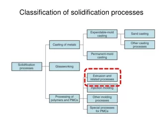
4. Basic aspects of alloy solidification a) Pure substance b) Binary alloy Liquidus interface Solid/liquid interface S O L I D M U S H Solidus interface LIQUID SOLID Liquid T T Tliq Tm Tsol x x

5. Important physical mechanisms in solidification Capillarity Dendrites movement Melt Double diffusive convection Solute Segregation Mushy Morphological instability Interfacial thermodynamics Solid Shrinkage Diffusion

6. Macrosegregation pattern in cast ingots V-segregation A-segregation • Macrosegregation refers • to mal-distribution of • alloy constituents • Length-scales ranging • from millimeters to • centimeters or even • meters • A consequence of • species advection in the • liquid Mold Casting Bottom negative cone segregation

7. Causes of melt flow in alloy solidification • Thermal and concentration gradients • Surface tension gradients at a free surface • Density changes due to solidification • Drag force from solid motion • Residual force due to filling of the mold • Electromagnetic field • External forces such as rotation of the mold

8. a) N > 0 b) -1 < N < 0 c) N < -1 L L L M M M S S S Thermosolutal convection in the melt N = RaC / RaT RaT = gβT∆TL3/ναRaC = gβC∆CL3/να

9. Relate previous works – two-domain model • Pioneering work by Flemings and coworkers in the • mid-1960s linking macrosegregation to • interdendritic fluid flow. • Mehrabian et al. extended Fleming’s work by • incorporating an equation for buoyancy-driven flow • in mushy region. • Fuji et al. refined the model by coupling the • momentum and energy equations. • The first model to couple the bulk melt and mushy • regions and to include macrosegregation was • reported by Ridder et al.

10. Limitation of the two-domain model • Explicit tracking of the phase • interfaces involved matching • variables at the boundaries. • Requires tracking of a • distinct solid/liquid interface, • which is very complex for • most alloy solidification • systems • Cannot predict phenomena • occurring in the mushy zone • such as channel formation, • remelting and double • diffusive interfaces. q • Macroscopic • scale (10-2~100m) L S (b) Microscopic scale (10-5~10-4m)

11. Relate previous works – single-domain model • Recent numerical investigation of metal alloy • solidification using single-domain model has been • done by Incropera et al. and Beckermann et al. • Advantages of single domain model include: • --- only a single set of equations to be solved in a single, fixed • numerical grid • --- phase interfaces are implicitly determined by the solution • of temperature and concentration fields • --- able to model freckle formation and remelting of solid • Two approaches to derive the single domain model: • --- volume averaging technique • --- classical continuum theory

12. Volume averaging technique Volume averaged quantity: Important theories: Mixture quantity: Ψ = <Ψl>*εl + <Ψs>*εs Solid Liquid Solid Liquid Definition of averaging volume О (l) << О(d) << О(L)

13. Assumptions for the volume averaged model • Only solid and liquid phases may be present • Variation in material properties are neglected in • averaging volume, although globally they may vary. • The flow is laminar and we assume Newtonian fluid. • The Boussinesq approximation is made • The solid phase is stationary • All the phases in the averaging volume are in • thermodynamical equilibrium • No back diffusion in the solid phase

14. Macroscopic governing equations

15. liquid Temperature liquidus Ti solidus α+liquid β+liquid α solid α+β solid eutectic point β solid Ci B A Concentration Supplementary relationships • Mixture enthalpy- liquid enthalpy relation • h = hl * εl + hs * εs • Mixture concentration–liquid concentration • relation (Lever rule) • C = Cl * εl+ Cs * εs • Thermodynamic relations (phase diagram) • C = [ (T - Tm)/(Te - Tm) ] *Ce

16. Finite element analysis – solution procedure start Go to next time step tn+1 Solve energy equation Decoupled solution methodology for various sub-problems at each time step Solve solute equation Solve momentum equations Update temperature, liquid concentration and volume fraction errors < tolerance? No yes

17. Finite element analysis – momentum equation • Stabilized finite element method (Tezduyar et al., 1990) • Darcy stabilizing term is added to the standard • SUPG/PSPG stabilizing method, velocity and pressure • are solved simultaneously, computationally intense • Penalty method (Brooks and Hughes, 1982) • eliminate pressure with the help of penalty function • and incorporate mass and momentum equations • into one equation • Fractional step method (Partankar, 1980) • solve velocity and pressure iteratively by projecting • velocity into divergence free function space

18. Stabilized finite element method The trial and test function spaces are defined as: The stabilized Galerkin formulation of the mass and momentum equations can be stated as follows:

19. Stabilized finite element method Where τSUPG and τPSPG are the standard SUPG and PSPG stabilizing parameters:

20. Stabilized finite element method • The spatial discretization of the weak form leads to • a set of nonlinear ordinary differential equation of • velocity and pressure. • The backward Euler method is utilized for time • stepping algorithm. • The resulting nonlinear algebraic equations are • solved by Newton’s method. • Due to the sparse nature of the resulting linear • system, an iterative solver (PrecondBiCGStab) is • used to reduce the computation cost.

21. Penalty method • Standard Garlerkin formulation is applied to the • modified momentum equation with the penalty term. • A 109 penalty number is chosen for all the examples. • Backward Euler time-marching scheme and • Newton’s method are used for solving the set of • nonlinear ODEs. • As the pressure is eliminated from the momentum • equation, the linear system to be solved is much • smaller than that of the stabilized method, so • Gaussian elimination is used for all examples.

22. Fractional step method Part one: obtain approximate pressure field Step 1: calculate fictitious velocity by dropping the pressure term in the momentum equation Step 2: extract pressure field from the fictitious velocity using Poisson equation

23. Fractional step method Part two: correct velocity and pressure iteratively Step 3: solve momentum equation for velocity using the newly obtained pressure field Step 4: solve Poisson equation for pressure correction and correct pressure as Step 5: velocity is correctly using the pressure correction

24. Finite element analysis – energy and solute equations • Energy equation • Solute equation • Standard form of scalar advection-diffusion equation

25. Example1: Natural convection in uniform porosity media 36 x 36 grid u = v = 0 y T = 1 u = v = 0 T = 0 u = v = 0 g ε = 0.8 x u = v = 0 Pr = 1 RaT = 108 Da = 7.8x10-8 a) streamline contour b) temperature contour

26. Example 2: double diffusive convection in uniform porosity media 50 x 50 grid u = v = 0 y T = 1 C = 1 u = v = 0 Pr = 1 RaT = 2x108 RaC = -1.8x108 Da = 7.4x10-7 T = 0 C = 0 u = v = 0 g ε = 0.6 u = v = 0 x c) isoconcentration a) streamline b) isotherm

27. Example 3: natural convection in variable porosity media u = v = 0 y 36 x 36 grid εw=0.4 Free Fluid ε = 1 T = 1 u = v = 0 T = 0 u = v = 0 x u = v = 0 Pr = 1 RaT = 106 Da = 6.6x10-7 a) streamline contour b) temperature contour

28. Example 4: directional binary alloy solidification y Material system Aqueous solution of ammonium chloride (NH4Cl-H2O) Finite element mesh 41 x 41 bilinear elements 1849 nodes Governing physical parameters Prandtl number 9.025 Lewis number 27.84 Darcy number 8.9x10-8 Thermal Rayleigh number 1.9x106 Solutal Rayleigh number -2.1x106 u = v = 0 ∂T/∂n = 0 ∂C /∂n = 0 u = v = 0 T = Tcold ∂C /∂n = 0 u = v = 0 T = Tinital ∂C /∂n = 0 H x L u = v = 0 ∂T/∂n = 0 ∂C /∂n = 0 Geometry, FE mesh and boundary conditions

29. Alloy solidification without convection

30. Alloy solidification with convection t* = 0.036 a) streamline b) isotherm c) isoconcentration a) streamline b) isotherm c) isoconcentration t* = 0.018

31. Alloy solidification with convection a) streamline b) isotherm c) isoconcentration Macrosegreation pattern at time t* = 0.14 Cinital = 0.7, Ceutectic = 0.803 t* = 0.07

32. Alloy solidification with convection

33. Effect of anisotropic permeability R = Kx / Ky = 4 Kx: permeability in the x direction Ky: permeability in the y direction t* = 0.036 a) streamline b) isotherm c) isoconcentration a) streamline b) isotherm c) isoconcentration t* = 0.018

34. Example 5: pure aluminum solidification q = 0 Bi Ta q = 0 g Melt Solid t* = 0.05 q = 0 1.0 Dimensionless physical parameters t* = 0.35

35. Conclusions for the numerical analysis of binary alloy solidification processes • Thermal-solutal convection is responsible • for macrosegregation • Permeability of the mushy zone will affect the • strength of flows in both mushy and bulk liquid • region as well as the shape of liquidus • Tested for a limiting case of pure substance • solidification, the single domain model demon- • strated great versatility

36. Suggestions for future studies • Additional physical phenomena • Thermo/diffusocapillary effect • Shrinkage • Electromagnetic field • Rotation and vibration • Multi-constituent alloys • Computational issues • Simulation of solidification system with higher • Rayleigh and Lewis number • Extend the model to 3D simulation • Parallelization of the program

37. Acknowledgements Thesis advisor: Professor Nicolas J. Zabaras Committee member: Professor Stephen A. Vavasis Discussions and motivations: Ganapathysubramanian Shankar Xiaoyi Li Research funded by a grant from NASA Additional support from Sibley School of Mechanical and Aerospace Engineering, Cornell University