Download
1 / 32
330 likes | 486 Vues
Introduction To Analog Filters. The University of Tennessee Knoxville, Tennessee. wlg. Filters. Background:. . Filters may be classified as either digital or analog. . Digital filters are implemented using a digital computer or special purpose digital hardware.

E N D
Introduction To Analog Filters The University of Tennessee Knoxville, Tennessee wlg
Filters Background: . Filters may be classified as either digital or analog. .Digital filters are implemented using a digital computer or special purpose digital hardware. . Analog filters may be classified as either passive or active and are usually implemented with R, L, and C components and operational amplifiers.
Filters Background: . An active filter is one that, along with R, L, and C components, also contains an energy source, such as that derived from an operational amplifier. . A passive filter is one that contains only R, L, and C components. It is not necessary that all three be present. L is often omitted (on purpose) from passive filter design because of the size and cost of inductors – and they also carry along an R that must be included in the design.
Filters Background: . The analysis of analog filters is well described in filter text books. The most popular include Butterworth, Chebyshev and elliptic methods. . The synthesis (realization) of analog filters, that is, the way one builds (topological layout) the filters, received significant attention during 1940 thru 1960. Leading the work were Cauer and Tuttle. Since that time, very little effort has been directed to analog filter realization.
Filters Background: . Generally speaking, digital filters have become the focus of attention in the last 40 years. The interest in digital filters started with the advent of the digital computer, especially the affordable PC and special purpose signal processing boards. People who led the way in the work (the analysis part) were Kaiser, Gold and Radar. . A digital filter is simply the implementation of an equation(s) in computer software. There are no R, L, C components as such. However, digital filters can also be built directly into special purpose computers in hardware form. But the execution is still in software.
Filters Background: . In this course we will only be concerned with an introduction to filters. We will look at both passive and active filters. . We will not cover any particular design or realization methods but rather use our understanding of poles and zeros in the s-plane. . All EE and CE undergraduate students should take a course in digital filter design, in my opinion.
Passive Analog Filters Four types of filters - “Ideal” Background: lowpass highpass bandpass bandstop
Passive Analog Filters Realistic Filters: Background: lowpass highpass bandpass bandstop
Passive Analog Filters Background: It will be shown later that the ideal filter, sometimes called a “brickwall” filter, can be approached by making the order of the filter higher and higher. The order here refers to the order of the polynomial(s) that are used to define the filter. Matlab examples will be given later to illustrate this.
Passive Analog Filters Low Pass Filter Consider the circuit below. + R + VI C VO _ _ Low pass filter circuit
Passive Analog Filters Low Pass Filter . 0 dB Bode -3 dB 1/RC Passes low frequencies Attenuates high frequencies 1 x Linear Plot 0.707 1/RC 0
Passive Analog Filters High Pass Filter Consider the circuit below. + C + R Vi VO _ _ High Pass Filter
Passive Analog Filters High Pass Filter 0 dB . -3 dB Passes high frequencies Bode 1/RC Attenuates low frequencies 1/RC 1 x . 0.707 Linear 0 1/RC
Passive Analog Filters Bandpass Pass Filter Consider the circuit shown below: + C L + VO Vi R _ _ When studying series resonant circuit we showed that;
Passive Analog Filters Bandpass Pass Filter We can make a bandpass from the previous equation and select the poles where we like. In a typical case we have the following shapes. 0 dB . . Bode -3 dB lo hi 1 . . 0.707 Linear lo hi 0
Passive Analog Filters Bandpass Pass Filter Example Suppose we use the previous series RLC circuit with output across R to design a bandpass filter. We will place poles at –200 rad/sec and – 2000 rad/sec hoping that our –3 dB points will be located there and hence have a bandwidth of 1800 rad/sec. To match the RLC circuit form we use: The last term on the right can be finally put in Bode form as;
Passive Analog Filters Bandpass Pass Filter Example From this last expression we notice from the part involving the zero we have in dB form; 20log(.0055) + 20logw Evaluating at w = 200, the first pole break, we get a 0.828 dB what this means is that our –3dB point will not be at 200 because we do not have 0 dB at 200. If we could lower the gain by 0.829 dB we would have – 3dB at 200 but with the RLC circuit we are stuck with what we have. What this means is that the – 3 dB point will be at a lower frequency. We can calculate this from
Passive Analog Filters Bandpass Pass Filter Example This gives an wlow = 182 rad/sec. A similar thing occurs at whi where the new calculated value for whi becomes 2200. These calculations do no take into account a 0.1 dB that one pole induces on the other pole. This will make wlo somewhat lower and whi somewhat higher. One other thing that should have given us a hint that our w1 and w2 were not going to be correct is the following: What is the problem with this?
Passive Analog Filters Bandpass Pass Filter Example The problem is that we have Therein lies the problem. Obviously the above cannot be true and that is why we have aproblem at the –3 dB points. We can write a Matlab program and actually check all of this. We will expect that w1 will be lower than 200 rad/sec and w2 will be higher than 2000 rad/sec.
Passive Analog Filters -3 dB -5 dB
A Bandpass Digital Filter Perhaps going in the direction to stimulate your interest in taking a course on filtering, a 10 order analog bandpass butterworth filter will be simulated using Matlab. The program is given below. N = 10; %10th order butterworth analog prototype [ZB, PB, KB] = buttap(N); numzb = poly([ZB]); denpb = poly([PB]); wo = 600; bw = 200; % wo is the center freq % bw is the bandwidth [numbbs,denbbs] = lp2bs(numzb,denpb,wo,bw); w = 1:1:1200; Hbbs = freqs(numbbs,denbbs,w); Hb = abs(Hbbs); plot(w,Hb) grid xlabel('Amplitude') ylabel('frequency (rad/sec)') title('10th order Butterworth filter')
RLC Band stop Filter Consider the circuit below: + R + L VO Vi _ C _ The transfer function for VO/Vi can be expressed as follows:
RLC Band Stop Filter Comments This is of the form of a band stop filter. We see we have complex zeros on the jw axis located From the characteristic equation we see we have two poles. The poles an essentially be placed anywhere in the left half of the s-plane. We see that they will be to the left of the zeros on the jw axis. We now consider an example on how to use this information.
RLC Band Stop Filter Example Design a band stop filter with a center frequency of 632.5 rad/sec and having poles at –100 rad/sec and –3000 rad/sec. The transfer function is: We now write a Matlab program to simulate this transfer function.
RLC Band Stop Filter Example num = [1 0 300000]; den = [1 3100 300000]; w = 1 : 5 : 10000; Bode(num,den,w)
RLC Band Stop Filter Example Bode Matlab
Basic Active Filters Low pass filter
Basic Active Filters High pass
Basic Active Filters Band pass filter
Basic Active Filters Band stop filter