Control by the Iron Fist: Modeling Biogeochemical Cycling in the Equatorial Pacific

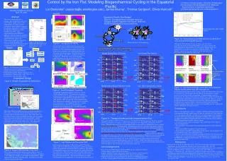
1. Control by the Iron Fist: Modeling Biogeochemical Cycling in the Equatorial Pacific -12.4 -7.5 -6.1 -0.7 -19.6 -3.1 -9.7 -20 3.7 0.3 1.9 1.7 0.44 0.3 0.1 3.4 3.7 7.3 0.2 1.9 PISCES (-0.1) (-5.5) (-0.7) (-1.1) 5.3 14.0 0.8 5.2 (-5.8) (0.1) (-3.0) (-12.4) 35.9 27.5 2.9 12.9 5°N positive anomaly 45m 45m 45m 45m 0.0 -0.2 1.1 -2.7 -0.9 -1.1 2.2 0.3 5°S 9.1 9.6 0.8 PO43- 0.1 1.0 0.0 0.2 2.5 6.4 5.3 0.5 3.2 Depth (m) Diatoms NH4+ negative anomaly 0.6 0.6 0.6 0.6 Si 17.7 14.2 7.3 1.4 34.9 31.4 13.1 4.1 Nano-phyto (0.2) (0.1) (1.5) (0.2) (0.0) (0.4) (0.0) (2.6) EUC NO3- 95m 95m 95m 95m Iron -1.4 -0.6 4.0 4.9 -0.6 -0.4 2.7 3.3 15.4 15.2 2.3 8.4 5.1 1.9 0.7 6.2 3.4 0.4 3.3 4.7 Remineralization (mol Fe*m-2s-1) Biology (mol Fe*mm-2s-1) Scavenging (mol Fe*mm-2s-1) MicroZoo Fe (nM) control run Fe (nM) 270m source 3.7 22.2 19.7 12.2 21.8 18.7 7.7 3.3 (1.6) (0.2) (3.2) (0.2) (0.0) (-0.3) (-0.7) (0.7) 180°W D.O.M 142m 142m 142m 142m 135°W 90°W Meso Zoo -1.9 -0.6 3.5 2.7 -0.3 0.1 2.5 0.9 4.8 21.1 21.5 17.9 18.9 3.4 18.5 8.3 0.9 0.2 0.6 0.2 12.5 14.3 3.0 5.0 7.3 1.7 4.6 1.5 P.O.M (0.0) (2.3) (1.5) (-0.5) (-1.1) (-5.1) (-5.5) (-2.2) 217m 217m 217m 217m Depth (m) Depth (m) 1.0 0.9 0.5 0.0 0.2 0.8 0.1 1.2 Small Big 11.8 3.0 11.7 5.0 0.35 0.6 0.3 2.0 1.9 0.2 0.5 0.1 0.3 [Fe] increase [NO3] increase [Fe] increase [NO3] increase (-0.7) (-2.6) (-1.4) (-2.9) 1.1 1.5 4.7 6.0 (-2.6) (-2.8) (-0.6) (-0.8) 1.4 6.5 1.4 6.9 272m 272m 272m 272m Fe (nM) Gordon et al. 180°W 180°W 180°W 180°W 134°W 134°W 134°W 134°W 90°W 90°W 90°W 90°W Biology Fe (nM) 180m source Fe Remineralization Scavenging Iron perturbation 180m Iron perturbation 270m control 154°-158°E, 0.5°S-0.5°N Mackey et al, 2002 Control 270m Source Levitus (1) School of Oceanography, University of Washington (2) Laboratoire d’Oceanographie et du Climat par Experimentation et Approche Numérique (3) Institut de Recherche pour le Développement Lia Ossiander1 (ossianla@u.washington.edu), James Murray1, Thomas Gorgues2, Olivier Aumont3 Graduate Climate ConferenceApril 7-9, 2006 Results Abstract Equatorial Pacific Box Budget The eastern equatorial Pacific is grazing- and iron-limited (Landry et al., 1997), but the supply of iron to this highly productive region is poorly constrained. Some evidence suggests a possible iron maximum in or just below the Equatorial Undercurrent (EUC) (Gordon et al., 1997). The biogeochemical model PISCES is applied to study the impact of candidate subsurface iron sources in the western equatorial Pacific. Iron in our simulations is rapidly scavenged from an eastward-moving plume, but exercises strong biogeochemical control on conditions in the eastern Pacific. Figure 8: Two approaches to calculate export flux, Transport Budget (Toggweiler and Carson, 1995) and PISCES biogeochemical sources and sinks World Ocean Atlas 2001 CSIRO archive Figure 10: Concentrations of Nitrate and Iron on 25.5 kg*m-3 on a zonal profile along the Equator. Figure 1: Gordon, Coale & Johnson 1997: Dissolved iron at 0, 140W with data from three cruises. Depth of EUC core varies temporally. dFe/dt = Physics + Netbiogeochem Figure 5: Iron profiles at 140°W Although the EUC provides the new nutrients to the east, nitrate concentrations of the eastward-flowing EUC water (represented by the 25.5 isopycnal) are relatively low (see red arrows in Figures 8 & 9) and are progressively enriched by respiration of organic material. The opposite trend is seen for iron, especially for the high initial iron concentrations in the 180m iron source run. An iron “bulls-eye” is visible in the two source runs, similar to the maximum observed in dissolved iron by Gordon et al. The simulated maximum is greater, due in part to the inclusion of acid-soluble particulate iron data in the western iron source. The black lines denote isopycnal surfaces. The EUC is visible in the doming of isopycnals. Model iron travels eastward along isopycnals and reaches the mixed layer in the eastern Pacific, although it is rapidly scavenged enroute. Biology = -1*(primary production Fe uptake – excretion) + zooplankton exudation Scavenging = 0.005d-1*(POCs + POCl + BSi)*(Fe-FeL) Remineralization = 0.1d-1*(0.25 + 0.75e -(z-zmel)/1000)*pFes Model OPA Iron Control Run (mol/s) Nitrate Control Run (104 mol/s) Control Figure 2: Saved dynamical fields from the OPA general circulation model with climatlogical forcing were used to run the PISCES biogeochemical model. Model resolution is 0.5˚ meridional near Equator and 2˚ zonal. There are 31 vertical levels, with 12 in upper 120m Depth (m) note difference in scales for scavenging Longitude Longitude Nanoplankton, control Nanoplankton, 270m source-control Experiment Design 180m Source Figure 3: Western Equatorial Iron Perturbation Depth (m) Nitrate 180 m Source Run (104 mol/s) Iron 180 m Source Run (mol/s) Longitude Longitude Figure 11: Iron biogeochemical source/sink terms along the Equator for the control and 180 m source run. Diatom Biomass, control Diatoms, 270m source-control Figure 6: Zonal Ecosystem Response The biogeochemical pathway of iron changes significantly between the control and 180 m source run, with the most dramatic shift in scavenging fluxes, which increase by more than an order of magnitude. Biological uptake is greatly increased near the surface in the source run, but decreases rapidly towards the base of euphotic zone and becomes a net positive source of iron by 140 m as a result of grazing-and bacterially-remediated remineralization. Remineralization from the small particulate iron pool exhibits a subsurface maximum just beneath the maximum biological uptake and also shows a corresponding increase in magnitude with the addition of a western iron source. Nanoplankton and Diatom biomass (μg/L) in a vertical section along the Equator. The stimulation in primary productivity driven by the additional iron upwelling in the eastern Pacific is apparent in the anomaly plots on the right. Diatoms show an especially strong response with a three-fold increase in biomass. Diatoms are less vulnerable to grazing pressure. Nanoplankton experience a smaller net biomass increase, but also an altered vertical distribution due to light limitation. The PISCES model does not resolve the diurnal cycle. Conclusions Three biogeochemical model runs were conducted with different iron sources: a control run with model default iron sources and two runs with an elevated western source. The 270m source was fit to Mackey et al.’s total acid-soluble iron data with a maximum below the core of the Equatorial Undercurrent (EUC) and the 180m source was placed in the core of the model’s EUC with a magnitude equal to that of the 270m source. All experiments were run 20-30 years, sufficient time for tropical Pacific biogeochemical equilibrium. • Data as to the distribution, sources, variability, and biogeochemical cycling of iron in the equatorial Pacific is quite sparse. In spite of (or because of?) this, modeling iron in the equatorial Pacific is a viable way to test the response of this productive ecosystem characterized by strong interannual variability. We’ve presented here the impact of hypothetical equatorial Pacific western-shelf iron sources within the PISCES biogeochemical model, and have shown: • A large western iron source can propagate across the Pacific basin, subject to large scavenging losses. • Iron availability exerts strong control on primary productivity and community structure. • The extent of HNLC conditions is regulated by iron. • Zonal transport in the EUC and upwelling are the primary nutrient pathways for new production in the eastern equatorial Pacific. • Nitrate is more efficiently recycled in the equatorial Pacific ecosystem than iron. • The fate of a western iron source is strongly dependent on scavenging rates. In the PISCES scavenging parameterization, iron scavenging is a dominant sink for the western source iron. Figure 9: Transport terms and net biogeochemical flux The central (180°W:134°W, 5°S:5°N) and eastern (134°W:90°W, 5°S:5°N) equatorial Pacific are divided into five vertical boxes for analysis, similar to the approach used by Toggweiler and Carson (1995) for nitrate. The zonal and vertical advective and diffusive fluxes into each box are depicted by arrows with the magnitude of the transport written in yellow. Meridional transports are relatively small, and are shown in parentheses in the lower left of each box. The nutrient budgets are at steady state, and the pink numbers in the upper right corner of each box show the net biogeochemical loss or gain of each nutrient, calculated by the net physical transport in or out of the box. Red arrows highlight those boxes for which the nutrient concentration increases along an isopycnal surface in the direction of flow. Isopycnal surfaces (matched to the depth of the boxes at 134°W) were used because the concentrations of all nutrients increases towards the east along a constant depth due to the eastward shoaling of the thermocline. Nitrate increases zonally, whereas iron does not (refer to Fig. 10). In the 180 m source run, the zonal transport of iron occurs shallower, due to the iron maximum directly in the core of EUC. Unlike in the control run, there is a net remineralization of iron in some of the shallower boxes. In contrast, nitrate is regenerated in all of the boxes below the euphotic zone in both the control and 180 m source run. 270 m control Levitus 180 m References Figure 7: High Nitrate Low Chlorophyll Shift Gordon, R. M., Coale, K.H., and Johnson, K.S. (1997) Iron distributions in the equatorial Pacific: Implications for new production. Limnology and Oceanography 42(3): 419-431 Landry et al. (1997) Iron and grazing constraints on primary production in the central equatorial Pacific: An EqPac synthesis. Limnology and Oceanography 42(3): 405-418. Mackey, D.J., O’Sullivan, J.E., and Watson, R.J. (2002) Iron in the western Pacific: a riverine or hydrothermal source for iron in the Equatorial Undercurrent? Deep-Sea Research I 49:877-893 Toggweiler, J.R. and Carson, S. (1995) What are Upwelling Systems Contributing to the Ocean’s Carbon and Nutrient Budgets? Upwelling in the Ocean: Modern Processes and Ancient Records 337-360. Surface nitrate concentrations (μM) for the control, 270 m iron source, and Levitus show that the addition of a western iron source reduces the magnitude and extent of HNLC conditions. The bottom left figure plots surface nitrate at the Equator for each of three model runs and Levitus. The control run achieves the high surface nitrate observed in the eastern Pacific, but overestimates nitrate over most of the central equatorial Pacific. The iron perturbations were upper-bound estimates for the magnitude of a western dissolved-iron source. Acknowledgements Merci beaucoup to Billy Kessler (NOAA, PMEL) for tips and tricks with Ferret and knowledge of equatorial Pacific dynamics. Graphics and analysis were made with the Ferret data analysis and visualization software developed at NOAA PMEL (http://ferret.pmel.noaa.gov/Ferret/). Funding for this project was provided by the University of Washington Program on Climate Change and the National Science Foundation grant OCE-0425721. Figure 4: August 2006 planned cruise track We will measure dissolved iron concentrations along a series of meridional transects aligned with the TOGA-TAO array and collect a suite of physical, biological, and chemical measurements. Model experiments help define sampling targets. Field data will be used to better constrain model input.