Download
1 / 36
370 likes | 467 Vues
Learn how to screen, explore, and clean up data for statistical analysis with detailed methods on descriptive statistics, measures of centrality and variability, handling outliers, and missing data.

E N D
“I Have a Bunch of Data – Now What?”Data Screening, Exploringand Clean-Up Melinda K. Higgins, Ph.D. 25 & 26 September 2008
Outline • Descriptive Statistics (univariate & bi-variate) • Measures of Centrality • Measures of Variability • Distributions & Transformations • Tests of Normality • Outliers • Missing Data • Correlations • Overall Flow Charts • Potential Statistical Analyses (Decision Tree) • Contact Info
A Few Initial Considerations • GROUPS – If data is to be evaluated by group – you will want to evaluate the descriptive statistics BY group (e.g. the data might not be skewed overall, but one group may be by itself) – may or may not want to transform. • LONGITUDINAL DATA – If variables were measured over time, you will need to consider all the time points (e.g. you would NOT want to transform one time point and not the others) • MULTIVARIATE MEASURES – additional screening measures in bi-variate/multivariate combinations (multicollinearity, influential cases, leverage, Mahalonobis distance) – not covered in this lecture.
Measures of Central Tendency • Mean = (Xi)/n • Median = 50% Below ≤ Median ≤ 50% Above • for odd n, Median=middle value(sorted X) • For even n, Median = average of 2 middle X’s • Trimmed Mean – mean recalculated after deleting _% or _# off top and bottom of sorted data (usually 5% or so) • Mode – number(s) repeated the most
Measures of Variance • (sample) Variance = sums of squares of deviation from mean/(n-1) • (sample) Standard Deviation = sqrt(variance) • Range = max(X) – min(X) • IQR – Interquartile Range = 75th Percentile(X) – 25th Percentile (X)
Distributions • Stem and Leaf • Dot plot • Histogram • Box plot
Boxplots (as Defined in SPSS) • A boxplot shows the five statistics (minimum, first quartile, median, third quartile, and maximum). It is useful for displaying the distribution of a scale variable and pinpointing outliers. • The boundaries of the box are “Tukey’s hinges.” The median is identified by a line inside the box. The length of the box is the interquartile range (IQR) computed from Tukey’s hinges [i.e. 25th and 75th percentiles]. • Outliers. Cases with values that are between 1.5 and 3 box lengths (box length=IQR) from either end of the box (“o”). Extremes. Cases with values more than 3 box lengths from either end of the box (“*”). • Whiskers at the ends of the box show the distance from the end of the box to the largest and smallest observed values that are less than 1.5 box lengths from either end of the box.
Distributions (cont’d) – Skewness and Kurtosis • Skewness and Kurtosis are the two most commonly used measures to evaluate deviations from normality. • Skewness measures the extent to which the distribution is not symmetric. • Kurtosis measure the extent to which the distribution is more “pointed/narrow” or “flatter/wider” than the normal distribution.
Statistical Test: Skewness & Kurtosis • Zs = (S_skew-0)/SE_skew • S_skew = Skewness measure • SE_skew is the std. error of skewness • Zk = (S_kurt-0)/SE_kurt • S_kurt = Kurtosis measure • SE_kurt is the std. error of kurtosis • Zs or Zk values > 1.96 are significant at 0.05 sig. level • Zs or Zk values > 2.58 are significant at 0.01 sig. level • Zs or Zk values > 3.29 are significant at 0.001 sig. level
Zs=103.08 Zs=7.3 Zk=990.98 Zk=2.7
Additional Tests of Normality • The following 2 tests compare the scores in the sample to a normally distributed set of scores with the same mean and std. deviation. If the test is non-significant (p<0.05) it says that the sample distribution is not significantly different from a normal population. • Kolmogorov-Smirov • Shapiro-Wilk • [NOTE: With larger sample sizes, these tests will be significant for small deviations from normality – use graphics/visual inspection.]
Transformations SPSS COMPUTE and/or SAS Data Procedure Moderate – positive skewness NEWX=SQRT(X) Substantial positive skewness NEWX=LG10(X) (with zero) NEWX=LG10(X+C) Severe positive skewness NEWX=1/X L-shaped (with zero) NEWX=1/(X+C) Moderate negative skewness NEWX=SQRT(K-X) Substantial negative skewness NEWX=LG10(K-X) Severe negative skewness (J-shaped) NEWX=1/(K-X) C = constant added so smallest score is 1 K = constant from which each score is subtracted so smallest score is 1.
LG10 Original SQRT
Outliers • Review histograms and boxplots and look for extreme values • Investigate values • is it “real?” • can it be corrected? • Should it be deleted (or left out of analyses)? • [consider clinical reasons; procedural reasons] • Calculate z-scores (next page) and review amount of outliers • Is there a pattern? (compare outliers to non-outliers)
Outliers DESCRIPTIVES VARIABLES=day2/SAVE. COMPUTE outlier1=abs(zday2). EXECUTE. RECODE outlier1 (3.29 thru Highest = 4) (2.58 thru highest = 3) (1.96 thru Highest = 2) (Lowest thru 2 = 1). EXECUTE. VALUE LABELS outlier1 1 'Absolute z-score less than 2' 2 'Absolute z-score greater than 1.96' 3 'Absolute z-score greater than 2.58' 4 'Absolute z-score greater than 3.29'. FREQUENCIES VARIABLES=outlier1. /ORDER=ANALYSIS. /SAVE option creates z-score of “DAY2”
Missing Data • Look for patterns (MVA next slide) and/or reason why missing • Can compare missing data subjects to non-missing data subjects • Can delete/ignore or Impute based on model • Goal is to: • Minimize Bias • Maximize utilization of information (data=$$) • Get good estimates of uncertainty • Censorship (survival analysis – “loss to follow-up”) • [SIDE NOTE: SPSS missing – strings vs. numeric data types] NOTE: Missing Data Imputation – to be discussed in another lecture
Missing Data MVA VARIABLES = timedrs attdrug atthouse income emplmnt mstatus race /TTEST PROB PERCENT=5 /MPATTERN /EM. None are significant (as compared to “INCOME”)
95 81 We fixed “m” but what about the subject with no gender (missing)? 1 1 (string) (numeric)
1 case not counted!! Case correctly counted This was an interesting case as designation of “anemia” depended only on age (if less than 12), but depends on both age and gender if older than 12. [Our missing gender was 8 yrs old.]
Measures of Correlation • [Parametric] R2 and R (X vs Y or X1 vs X2) = Pearson's correlation coefficient • [Non-parametric] Spearman's rho, and Kendall's tau-b – both based on rank (see SPSS Help for further details)
Checklist for Data Screening • Inspect univariate descriptive stats – check for data accuracy/discrepancies • Out-of-range values • Plausible means and standard deviations • Univariate outliers • Evaluate amount and patterns of missing data • Check pairwise plots for nonlinearity and heteroscedasticity [REGRESSION] • Identify and deal with nonnormal variables and univariate outliers • Check skewness and kurtosis and probability plots • Perform transforms (if desired) • Check results of transformation • Identify multivariate outliers [REGRESSION] • Evaluate variables for multicollinearity and singularity [REGRESSION]
What do I do Now? – A Decision Tree for Picking Statistical Methods to Use • Questions to Ask • Major Research Question? • Degree of Relationship Among Variables • Significant Group Difference • Prediction of Group Membership • Structure • Time/Course of Events • Number & Kind of Dependent Variables • Single vs Multiple & Discrete vs Continuous • Number & Kind of Independent Variables • Single vs Multiple & Discrete vs Continuous • Covariates? [yes/no] • Decision Tree Yields Analytic Strategy and Goal of Analysis
Tabachnick, B.G. and Fidell, L.S. (2007) Using Multivariate Statistics (5th Ed.). New York: Pearson Education, Inc.
“How to talk to a Statistician” • List of Hypotheses/Aims (end goals) • List of Variables • Type, Measure (numeric, string, date/time, scales, categorical) • Independent, covariates, dependent (outcomes) • Names, Labels and Values [consistency (q1,q2,q3,…, item01,item02,…), length, consider graphics] • Model (hypothesized, general idea – theoretical concerns) • Graphics/figures/tables requested (reports, posters, grants) • POWER – idea on “effect size” (how big a change do you hope to see) – clinical significance, prior results?
SON S:\Shared\Statistics_MKHiggins\website2\index.htm [updates in process] Working to include tip sheets (for SPSS, SAS, and other software), lectures (PPTs and handouts), datasets, other resources and references Statistics At Nursing Website: [website being updated] http://www.nursing.emory.edu/pulse/statistics/ And Blackboard Site (in development) for “Organization: Statistics at School of Nursing” Contact Dr. Melinda Higgins Melinda.higgins@emory.edu Office: 404-727-5180 / Mobile: 404-434-1785 VIII. Statistical Resources and Contact Info