Evaluation - Controlled Experiments
Evaluation - Controlled Experiments. What is experimental design? What is an experimental hypothesis? How do I plan an experiment? Why are statistics used? What are the important statistical methods?.

Evaluation - Controlled Experiments
E N D
Presentation Transcript
Evaluation - Controlled Experiments What is experimental design? What is an experimental hypothesis? How do I plan an experiment? Why are statistics used? What are the important statistical methods? Slide deck by Saul Greenberg. Permission is granted to use this for non-commercial purposes as long as general credit to Saul Greenberg is clearly maintained. Warning: some material in this deck is used from other sources without permission. Credit to the original source is given if it is known.
Quantitative evaluation of systems • Quantitative: • precise measurement, numerical values • bounds on how correct our statements are • Methods • user performance data collection • controlled experiments
Collecting user performance data • Data collected on system use (often lots of data) • Exploratory: • hope something interesting shows up • but difficult to analyze • Targeted • look for specific information, but may miss something • frequency of request for on-line assistance • what did people ask for help with? • frequency of use of different parts of the system • why are parts of system unused? • number of errors and where they occurred • why does an error occur repeatedly? • time it takes to complete some operation • what tasks take longer than expected?
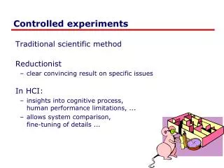
Controlled experiments • Traditional scientific method • Reductionist • clear convincing result on specific issues • In HCI: • insights into cognitive process, human performance limitations, ... • allows system comparison, fine-tuning of details ...
Controlled experiments • Strives for lucid and testable hypothesis quantitative measurement measure of confidence in results obtained (statistics) replicability of experiment control of variables and conditions removal of experimenter bias
A) Lucid and testable hypothesis • State a lucid, testable hypothesis • this is a precise problem statement • Example 1: There is no difference in the number of cavities in children and teenagers using crest and no-teeth toothpaste when brushing daily over a one month period
File Edit View Insert File New Edit New Open Open View Close Insert Close Save Save A) Lucid and testable hypothesis • Example 2: There is no difference in user performance (time and error rate) when selecting a single item from a pop-up or a pull down menu of 4 items, regardless of the subject’s previous expertise in using a mouse or using the different menu types”
Independent variables • b) Hypothesis includes the independent variables that are to be altered • the things you manipulate independent of a subject’s behaviour • determines a modification to the conditions the subjects undergo • may arise from subjects being classified into different groups
Independent variables • in toothpaste experiment • toothpaste type: uses Crest or No-teeth toothpaste • age: <= 11 years or > 11 years • in menu experiment • menu type: pop-up or pull-down • menu length: 3, 6, 9, 12, 15 • subject type (expert or novice)
Dependant variables • c) Hypothesis includes the dependent variables that will be measured • variables dependent on the subject’s behaviour / reaction to the independent variable • the specific things you set out to quantitatively measure / observe
Dependant variables • in menu experiment • time to select an item • selection errors made • time to learn to use it to proficiency • in toothpaste experiment • number of cavities • frequency of brushing • preference
Subject Selection • d) Judiciously select and assign subjects to groups • ways of controlling subject variability • reasonable amount of subjects • random assignment • make different user groups an independent variable • screen for anomalies in subject group • superstars versus poor performers Novice Expert
Controlling bias • e) Control for bias • unbiased instructions • unbiased experimental protocols • prepare scripts ahead of time • unbiased subject selection Now you get to do the pop-up menus. I think you will really like them... I designed them myself!
Statistical analysis • f) Apply statistical methods to data analysis • confidence limits: • the confidence that your conclusion is correct • “the hypothesis that computer experience makes no difference is rejected at the .05 level”means: • a 95% chance that your statement is correct • a 5% chance you are wrong
Interpretation • g) Interpret your results • what you believe the results really mean • their implications to your research • their implications to practitioners • how generalizable they are • limitations and critique
Planning flowchart for experiments Stage 1 Stage 2 Stage 3 Stage 4 Stage 5 Problem Planning Conduct Analysis Interpret- definition research ation feedback research define data interpretation preliminary idea variables reductions testing generalization literature review controls statistics data reporting collection apparatus hypothesis statement of testing problem procedures hypothesis select development subjects experimental design feedback Copied from an early ACM CHI tutorial, but I cannot recall which one
Statistical analysis • Calculations that tell us • mathematical attributes about our data sets • mean, amount of variance, ... • how data sets relate to each other • whether we are “sampling” from the same or different distributions • the probability that our claims are correct • “statistical significance”
Statistical vs practical significance • When n is large, even a trivial difference may show up as a statistically significant result • eg menu choice: mean selection time of menu a is 3.00 seconds; menu b is 3.05 seconds • Statistical significance does not imply that the difference is important! • a matter of interpretation • statistical significanceoften abused and used to misinform
Example: Differences between means Condition one: 3, 4, 4, 4, 5, 5, 5, 6 • Given: • two data sets measuring a condition • height difference of males and females • time to select an item from different menu styles ... • Question: • is the difference between the means of this data statistically significant? • Null hypothesis: • there is no difference between the two means • statistical analysis: • can only reject the hypothesis at a certain level of confidence Condition two: 4, 4, 5, 5, 6, 6, 7, 7
mean = 4.5 Example: 3 • Is there a significant difference between these means? 2 1 Condition one: 3, 4, 4, 4, 5, 5, 5, 6 0 3 4 5 6 7 Condition 1 Condition 1 3 mean = 5.5 2 1 Condition two: 4, 4, 5, 5, 6, 6, 7, 7 0 3 4 5 6 7 Condition 2 Condition 2
Problem with visual inspection of data • Will almost always see variation in collected data • Differences between data sets may be due to: • normal variation • eg two sets of ten tosses with different but fair dice • differences between data and means are accountable by expected variation • real differences between data • eg two sets of ten tosses for with loaded dice and fair dice • differences between data and means are not accountable by expected variation
T-test • A simple statistical test • allows one to say something about differences between means at a certain confidence level • Null hypothesis of the T-test: • no difference exists between the meansof two sets of collected data • possible results: • I am 95% sure that null hypothesis is rejected • (there is probably a true difference between the means) • I cannot reject the null hypothesis • the means are likely the same
Different types of T-tests • Comparing two sets of independent observations • usually different subjects in each group • number per group may differ as well Condition 1 Condition 2 S1–S20 S21–43 • Paired observations • usually a single group studied under both experimental conditions • data points of one subject are treated as a pair Condition 1 Condition 2 S1–S20 S1–S20
Different types of T-tests • Non-directional vs directional alternatives • non-directional (two-tailed) • no expectation that the direction of difference matters • directional (one-tailed) • Only interested if the mean of a given condition is greater than the other
T-test... • Assumptions of t-tests • data points of each sample are normally distributed • but t-test very robust in practice • population variances are equal • t-test reasonably robust for differing variances • deserves consideration • individual observations of data points in sample are independent • must be adhered to • Significance level • decide upon the level before you do the test! • typically stated at the .05 or .01 level
Two-tailed unpaired T-test • N: number of data points in the one sample • SX: sum of all data points in one sample • X: mean of data points in sample • S(X2): sum of squares of data points in sample • s2: unbiased estimate of population variation • t: t ratio • df = degrees of freedom = N1 + N2 – 2 • Formulas
Level of significance for two-tailed test df .05 .01 1 12.706 63.657 2 4.303 9.925 3 3.182 5.841 4 2.776 4.604 5 2.571 4.032 6 2.447 3.707 7 2.365 3.499 8 2.306 3.355 9 2.262 3.250 10 2.228 3.169 11 2.201 3.106 12 2.179 3.055 13 2.160 3.012 14 2.145 2.977 15 2.131 2.947 df .05 .01 16 2.120 2.921 18 2.101 2.878 20 2.086 2.845 22 2.074 2.819 24 2.064 2.797
Example Calculation x1 = 3 4 4 4 5 5 5 6 Hypothesis: there is no significant difference x2 = 4 4 5 5 6 6 7 7 between the means at the .05 level Step 1. Calculating s2
Example Calculation Step 2. Calculating t
Example Calculation df .05 .01 1 12.706 63.657 … 142.1452.977 15 2.131 2.947 • Step 3: Looking up critical value of t • Use table for two-tailed t-test, at p=.05, df=14 • critical value = 2.145 • because t=1.871 < 2.145, there is no significant difference • therefore, we cannot reject the null hypothesis i.e., there is no difference between the means
Two-tailed Unpaired T-test Or, use a statistics package (e.g., Excel has simple stats) Condition one: 3, 4, 4, 4, 5, 5, 5, 6 Condition two: 4, 4, 5, 5, 6, 6, 7, 7 Unpaired t-test Prob. (2-tail): DF: Unpaired t Value: 14 -1.871 .0824 Group: Count: Mean: Std. Dev.: Std. Error: one 8 4.5 .926 .327 two 8 5.5 1.195 .423
Significance levels and errors • Type 1 error • reject the null hypothesis when it is, in fact, true • Type 2 error • accept the null hypothesis when it is, in fact, false • Effects of levels of significance • high confidence level (eg p<.0001) • greater chance of Type 2 errors • low confidence level (eg p>.1) • greater chance of Type 1 errors • You can ‘bias’ your choice depending on consequence of these errors
Type I and Type II Errors • Type 1 error • reject the null hypothesis when it is, in fact, true • Type 2 error • accept the null hypothesis when it is, in fact, false Decision “Reality”
7 5 9 Example: The SpamAssassin Spam Rater • A SPAM rater gives each email a SPAM likelihood • 0: definitely valid email… • 1: • 2: … • 9: • 10: definitely SPAM SPAM likelihood 1 Spam Rater 3 7
7 5 9 Example: The SpamAssassin Spam Rater • A SPAM assassin deletes mail above a certain SPAM threshold • what should this threshold be? • ‘Null hypothesis’: the arriving mail is SPAM <=X 1 Spam Rater 3 7 >X
7 5 9 Example: The SpamAssassin Spam Rater • Low threshold = many Type I errors • many legitimate emails classified as spam • but you receive very few actual spams • High threshold = many Type II errors • many spams classified as email • but you receive almost all your valid emails <=X 1 Spam Rater 3 7 >X
Which is Worse? • Type I errors are considered worse because the null hypothesis is meant to reflect the incumbent theory. • BUT • you must use your judgement to assess actual risk of being wrong in the context of your study.
New Open Close Close Open New Save Save Significance levels and errors • There is no difference between Pie and traditional pop-up menus • What is the consequence of each error type? • Type 1: • extra work developing software • people must learn a new idiom for no benefit • Type 2: • use a less efficient (but already familiar) menu • Which error type is preferable? • Redesigning a traditional GUI interface • Type 2 error is preferable to a Type 1 error • Designing a digital mapping application where experts perform extremely frequent menu selections • Type 1 error preferable to a Type 2 error
Scales of Measurements • Four major scales of measurements • Nominal • Ordinal • Interval • Ratio
Nominal Scale • Classification into named or numbered unordered categories • country of birth, user groups, gender… • Allowable manipulations • whether an item belongs in a category • counting items in a category • Statistics • number of cases in each category • most frequent category • no means, medians… With permission of Ron Wardell
Nominal Scale • Sources of error • agreement in labeling, vague labels, vague differences in objects • Testing for error • agreement between different judges for same object With permission of Ron Wardell
Ordinal Scale • Classification into named or numbered ordered categories • no information on magnitude of differences between categories • e.g. preference, social status, gold/silver/bronze medals • Allowable manipulations • as with interval scale, plus • merge adjacent classes • transitive: if A > B > C, then A > C • Statistics • median (central value) • percentiles, e.g., 30% were less than B • Sources of error • as in nominal With permission of Ron Wardell
Interval Scale • Classification into ordered categories with equal differences between categories • zero only by convention • e.g. temperature (C or F), time of day • Allowable manipulations • add, subtract • cannot multiply as this needs an absolute zero • Statistics • mean, standard deviation, range, variance • Sources of error • instrument calibration, reproducibility and readability • human error, skill… With permission of Ron Wardell
Ratio Scale • Interval scale with absolute, non-arbitrary zero • e.g. temperature (K), length, weight, time periods • Allowable manipulations • multiply, divide With permission of Ron Wardell
Example: Apples • Nominal: • apple variety • Macintosh, Delicious, Gala… • Ordinal: • apple quality • US. Extra Fancy • U.S. Fancy, • U.S. Combination Extra Fancy / Fancy • U.S. No. 1 • U.S. Early • U.S. Utility • U.S. Hail With permission of Ron Wardell
Example: Apples • Interval: • apple ‘Liking scale’ Marin, A. Consumers’ evaluation of apple quality. Washington Tree Postharvest Conference 2002. After taking at least 2 bites how much do you like the apple? Dislike extremely Neither like or dislike Like extremely • Ratio: • apple weight, size, … With permission of Ron Wardell
Correlation • Measures the extent to which two concepts are related • eg years of university training vs computer ownership per capita • How? • obtain the two sets of measurements • calculate correlation coefficient • +1: positively correlated • 0: no correlation (no relation) • –1: negatively correlated
10 9 8 7 6 5 4 3 2.5 3 3.5 4 4.5 5 5.5 6 6.5 7 7.5 Correlation r2 = .668 condition 1 condition 2 5 6 4 5 6 7 4 4 5 6 3 5 5 7 4 4 5 7 6 7 6 6 7 7 6 8 7 9 Condition 1 Condition 1
Correlation • Dangers • attributing causality • a correlation does not imply cause and effect • cause may be due to a third “hidden” variable related to both other variables • drawing strong conclusion from small numbers • unreliable with small groups • be wary of accepting anything more than the direction of correlation unless you have at least 40 subjects
10 9 8 7 6 5 4 3 2.5 3 3.5 4 4.5 5 5.5 6 6.5 7 7.5 Correlation r2 = .668 Pickles eaten per month Salary per year (*10,000) 5 6 4 5 6 7 4 4 5 6 3 5 5 7 Salary per year (*10,000) 4 4 5 7 6 7 6 6 7 7 6 8 7 9 Which conclusion could be correct?-Eating pickles causes your salary to increase -Making more money causes you to eat more pickles -Pickle consumption predicts higher salaries because older people tend to like pickles better than younger people, and older people tend to make more money than younger people Pickles eaten per month