Analyzing Time-Dependent Acceleration in Motion Dynamics
This resource explores the complexities of motion when acceleration is not constant. Unlike previous studies which assume constant acceleration, this text delves into scenarios where acceleration varies with time. By examining a body subjected to multiple time-dependent force vectors, we derive the equations of motion for each direction. This includes calculating velocity and position vectors through integration of acceleration over time. The final position vector is presented as a function of time, demonstrating the intricate relationship between forces and motion in three-dimensional space.

Analyzing Time-Dependent Acceleration in Motion Dynamics
E N D
Presentation Transcript
Motion III Acceleration is not constant
Up until now, we have only considered motion where the acceleration is constant with respect to time. • Now let us consider the general case of time dependent acceleration.
Forces on a Body • Consider a body of mass m subject to many time dependent force vectors. • Taking the vector sum of all the force vectors applied to the body, we get • Σ F = (t + 1)i + (t2 + 3t – 4)j + (2)k • a = [(t + 1)/m]i+ [(t2 + 3t – 4)/m]j +(2/m)k • Motion in each direction is independent of motion in the other directions, so
ax= [(t + 1)/m]i • ay= [(t2 + 3t – 4)/m]j • az= (2/m)k • Remembering that ∫dv = ∫adt • We can integrate the left side from voto v • And the right side from toto t. • For the x, the y, and the z directions, but a must be kept inside the integral because it is time dependent!
vx= vox + ∫[(t + 1)/m]idt • vx= vox+ (1/m)[(t2/2) + t]i • vy= voy+ ∫[( t2 + 3t – 4)/m]jdt • vy= voy+ (1/m)[(t3/3) + (3t2/2) – 4t]j • vz= voz + ∫[(-4)/m]kdt • vz= voz - (4t)/m]k
The three dimensional velocity vector equation is now: • v = vx + vy + vz • v = vox+ (1/m)[(t2/2) + t]i+ voy+ (1/m)[(t3/3) + (3t2/2) – 4t]j + voz- (4t)/m]k
To obtain the position vectors x, y, z, one must integrate again • ∫dx = ∫vxdt • x = xo+ ∫{vox+ (1/m)[(t2/2) + t]i}dt • x = xo+ voxt + (1/m)[(3t3/6) + (t2/2]i • ∫dy = ∫vydt • y = yo+ ∫{voy+ (1/m) )[(t3/3) + (3t2/2) – 4t]j}dt • y = yo+ voyt + (1/m) )[(t4/12) + (t3/2) – 2t2
∫dz = ∫vzdt • z = zo+ ∫{voz+ (1/m)[(-4 t]k}dt • z = zo+ vozt + (1/m)[(-2 t2]k
The final position vector r is a function of time and would be the vector sum • r = x + y + z • r = xo+ voxt + (1/m)[(3t3/6) + (t2/2]i+ yo+ voyt + (1/m) )[(t4/12) + (t3/2) – 2t2]j + zo+ vozt + (1/m)[(-2 t2]k