Reliability Considerations for Laser Driver Integration in Inertial Fusion Energy Systems
This work addresses the reliability of laser drivers used in the HAPL project, where the shot life is quantified between 10^8 to 10^9 shots, translating to approximately 270 to 2700 operational hours at 10 Hz. The focus is on determining individual unit operation duration and repair time to achieve system availability. By analyzing failure rates and integrating a Weibull distribution model, we outline how to establish subsystem reliability requirements and operational costs, all while learning from experiences with solid-state IFE storage lasers.

Reliability Considerations for Laser Driver Integration in Inertial Fusion Energy Systems
E N D
Presentation Transcript
UCRL-POST-213303 Laser Driver Reliability Considerations HAPL Integration Group Earl Ault June 20, 2005
Purpose of this work • So far the HAPL project has characterized the required reliability of the laser driver by a single number, the shot life in the range of 108 to 109 shots • At 10 Hz this translates into a “lifetime” of ~270 to ~2700 hours • This is a simplification; the real question is “How long does an individual unit (beam line) have to run and how long do we have to repair a unit in order to achieve an acceptable system availability ?” • In the work described below we deal with this question • Once we know the relationship between unit failure rate and system availability we can then establish the reliability requirements for an IFE driver at the subsystem level • From this we can determine how much it costs to run and repair the system at a given availability
Previous experience • Our experience in solid state IFE storage lasers is based on single shot systems where the issue is making sure nearly all the beam lines fire at the right time and with the right power balance • For a rep-rated system the additional requirement is availability, the fraction of the system that is online compared to its full up capacity • In the Mercury laser the main “unreliability” is caused by optical damage of critical components • Diodes, pin holes, transport optics, etc., are expected to fail gracefully, leading to degraded performance over time • Critical optical elements can be single point, catastrophic failures • In Mercury, comprehensive damage diagnostics allow us to intervene before catastrophic damage occurs • Repairs can be effected to mitigate the cost of full replacement once damage initiation is discovered, but at a cost in dollars and availability
Reliability Considerations • For the IFE driver we don’t yet know the characteristics • of these failures because we do not have design and • testing information • What we can do is to use simple tools to understand what is required of these designs and see the impact of system • architecture decisions • For this poster we will assume that testing has caught most infant failures and the design is robust enough to have a low random failure component • We assume the operations management is sufficiently mature that failures due to operator errors or QC problems are rare • This leaves some sort of wear out failure, e.g., critical optical component damage, etc.
Wear out or lifetime failures Different failure distributions Wear out failure Infant failure MTBF Random failures
IRE Plant Driver Simulator • A numerical simulator is used to clock through system operating hours with failed units dropping out and being repaired and coming back on-line • NIF like architecture - 192 beam lines • Assumptions: • All beam lines identical • Beam lines are grouped in quads (4) for delivery the the target • Have a Mean Time Before Failure that can be characterized by a Weibull distribution • Repair time equals clock tic time • System availability defined as units running divided by units installed • Two cases are considered: service by quad (repair 1, idle 3) and repair single beam lines while all others run normally
Weibull Distribution Reliability function R = e-(t^) / • Well behaved function, found to be appropriate for complex systems characterized by a life time • We define the characteristic time as the MTBF • is a shape factor • =1 defines an exponential distribution • We use in the range of 6-10 to get a smeared out failure probability to model the statistical effect of beam lines having a distribution of life times around some mean life time
Weibull distribution continued R = e-(t^)/
Probability Matrix R = e-(t^)/ • We need to find a way to distribute the possible failure times of an ensemble of beam lines all running at the same time • Form a matrix of rows equal to a reliability value and columns related to the age of the device • For reliability values greater than R assign a one • For values less than R assign a zero • Select elements by asking the question “At a given age, what is the reliability value?” Select a value at random from the total available row values. If the element is 1, continue running. If zero, declare a failure and repair.
Probability Matrix continued R = e-(t^)/ 1111111111000000000000000 1111111111100000000000000 1111111111110000000000000 1111111111110000000000000 1111111111111000000000000 1111111111111000000000000 1111111111111100000000000 1111111111111111000000000 1111111111111111111000000 Create a matrix of 10,000 elements For this model 100 rows (related to Probability) 100 columns (related to time)
Test of the Probability Matrix Define as MTBF (probibility = 1/e) 20,000 tries at randomly selecting matrix elements shows that the 10,000 element probability matrix displays the desired shape of a Weibull distribution
Run model • The model consists of a matrix of cells, each is a beam line • The accumulated running hours on that line since the last repair is shown in the cell • A running cell is green • An idle cell is yellow • A failed cell is red • The program updates each cell by a tic equal to the MTTR (not required, could by any time step) • Each cell is interrogated and the run time compared to the probability matrix to see if it should fail or not • On the next tic all the units are back in service • We keep track of the total failures, integrated failures, and availability • Operating costs can then be estimated based on repair cost and number of units per day repaired Quad Port bundle of single lines Beam line age hr
Comments concerning the previous slides • The peaks and valleys in availability as well as in the number of failures is an artifact of the system being activated 4 beams at a time. Over time they smear out as the individual beam ages become random. • The failures begin to show up at a few hundred hours because the system is activated in groups every 10 hours. Therefore there is a range of ages when we start the clock • The dips in availability are significant and would likely require the plant to be out of service for the repair time (5 hr in this example) • Even with a MTTB of 1000 hours or 3.6x10⁶ shots with a fairly broad Weibull distribution of failure life times as this example shows, system availability is over 90% most of the time • If the distribution of the failures can be narrowed (a steeper Weibull centered at a given age) then is is possible to have a preventative maintenance program that could synchronize repairs with other plant activities so as to achieve higher availability when the driver is operating
Model results with beams repaired individually • Target symmetry will likely require fewer out of service beams than shown in the first case • This can be addressed by designing the system to allow single beam line repair, increase the individual reliability,or both • Here we have relaxed the requirement to idle 3 beams when repairing a single beam while leaving the MTBF and MTTR the same • We see that the availability is significantly improved, never dipping below 95% • Even with an MTBF of 1000 hr (3.6x10⁶ shots) driver performance may be adequate in terms of beam balance • Obviously extended shot life and the possibility of a preventative maintenance program will reduce costs and down time
Summary • The minimum availability the plant can tolerate will depend on the beam bundling architecture, power balance on target, and beam symmetry • Integration choices and selection of LRU unit design are important issues that ultimately drive system performance • This tool allows us to study these questions and can be extended to the reliability assessment at the beam line or lower level • In addition, the simulator gives us a way to partition the system into appropriate LRUs for optimum repair and operation • With these two simple examples we see the impact of the decision to repair at the quad level as in a NIF architecture (4 beams, 3 idle, 1 repaired) verses ability to repair at the single beam level