Tidal Flat Morphodynamics: A Synthesis
320 likes | 545 Vues
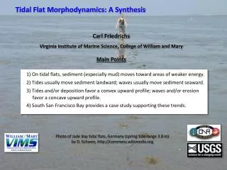
Tidal Flat Morphodynamics: A Synthesis. Carl Friedrichs Virginia Institute of Marine Science, College of William and Mary Main Points. 1) On tidal flats, sediment (especially mud) moves toward areas of weaker energy.

Tidal Flat Morphodynamics: A Synthesis
E N D
Presentation Transcript
Tidal Flat Morphodynamics: A Synthesis Carl Friedrichs Virginia Institute of Marine Science, College of William and Mary Main Points 1) On tidal flats, sediment (especially mud) moves toward areas of weaker energy. 2) Tides usually move sediment landward; waves usually move sediment seaward. 3) Tides and/or deposition favor a convex upward profile; waves and/or erosion favor a concave upward profile. 4) South San Francisco Bay provides a case study supporting these trends. Photo of Jade Bay tidal flats, Germany (spring tide range 3.8 m) by D. Schwen, http://commons.wikimedia.org
Tidal Flat Definition and General Properties e.g., Yangtze mouth (a) Open coast tidal flat Tidal flat = low relief, unvegetated, unlithified region between highest and lowest astronomical tide. e.g., Dutch Wadden Sea (b) Estuarine or back-barrier tidal flat (Sketches from Pethick, 1984) 1/17
Tidal Flat Definition and General Properties e.g., Yangtze mouth (a) Open coast tidal flat Tidal flat = low relief, unvegetated, unlithified region between highest and lowest astronomical tide. Note there are no complex creeks or bedforms on these simplistic flats. e.g., Dutch Wadden Sea (b) Estuarine or back-barrier tidal flat (Sketches from Pethick, 1984) 1/17
Where do tidal flats occur? According to Hayes (1979), flats are likely in “tide-dominated” conditions, i.e., Tidal range > ~ 2 to 3 times wave height. Tide-Dominated (High) Tide-Dominated (Low) Mixed Energy (Tide-Dominated) Mean tidal range (cm) Mixed Energy (Wave-Dominated) Wave-Dominated Mean wave height (cm) 2/17
What moves sediment across flats? Tidal advection High energy waves and/or tides Low energy waves and/or tides Higher sediment concentration 3/17
What moves sediment across flats? Ans: Tides plus energy-driven concentration gradients Tidal advection High energy waves and/or tides Low energy waves and/or tides Higher sediment concentration Tidal advection High energy waves and/or tides Low energy waves and/or tides Lower sediment concentration 3/17
< What moves sediment across flats? Ans: Tides plus energy-driven concentration gradients or supply-driven Tidal advection High energy waves and/or tides Low energy waves and/or tides Higher sediment concentration Tidal advection High energy waves and/or tides Low energy waves and/or tides Lower sediment concentration 3/17
Typical sediment grain size and tidal velocity pattern across tidal flats: Mud is concentrated near high water line where tidal velocities are lowest. Ex. Jade Bay, German Bight, mean tide range 3.7 m; Spring tide range 3.9 m. 5 km Photo location 1 m/s 0.25 0.50 1.00 1.50 Fine sand Sandy mud Mud Umax (m/s) (Grabemann et al. 2004) (Reineck 1982) 4/17
Typical sediment grain size and tidal velocity pattern across tidal flats: Mud is concentrated near high water line where tidal velocities are lowest. Ex. Jade Bay, German Bight, mean tide range 3.7 m; Spring tide range 3.9 m. 5 km Photo location 1 m/s 0.25 0.50 1.00 1.50 Fine sand Sandy mud Mud Umax (m/s) (Grabemann et al. 2004) (Reineck 1982) 4/17
Tidal Flat Morphodynamics: A Synthesis Carl Friedrichs and Josh Bearman Virginia Institute of Marine Science, College of William and Mary Main Points 1) On tidal flats, sediment (especially mud) moves toward areas of weaker energy. 2) Tides usually move sediment landward; waves usually move it seaward. 3) Tides and/or deposition favor a convex upward profile; waves and/or erosion favor a concave upward profile. 4) South San Francisco Bay provides a case study supporting these trends. Photo of Jade Bay tidal flats, Germany (spring tide range 3.8 m) by D. Schwen, http://commons.wikimedia.org
1 km 1 km Following energy gradients: Storms move sediment from flat to sub-tidal channel; Tides move sediment from sub-tidal channel to flat Ex. Conceptual model for flats at Yangtze River mouth (mean range 2.7 m; spring 4.0 m) Study Site 0 20 km (Yang, Friedrichs et al. 2003) Spring High Tide (+4 m) Storm-Induced High Water (+5 m) Spring Low Tide (0 m) Spring Low Tide (0 m) (a) Response to Storms (b) Response to Tides 5/17
Maximum tide and wave orbital velocity distribution across a linearly sloping flat: z = R/2 h(t) = (R/2) sin wt x = L Z(x) h(x,t) z = 0 (Friedrichs, in press) z = - R/2 x = 0 x x = xf(t) Spatial variation in tidal current magnitude 1.4 1.2 1.0 0.8 0.6 0.4 0.2 UT90/UT90(L/2) Landward Tide-Induced Sediment Transport 0 0.2 0.4 0.6 0.8 1 x/L 6/17
Maximum tide and wave orbital velocity distribution across a linearly sloping flat: z = R/2 h(t) = (R/2) sin wt x = L Z(x) h(x,t) z = 0 (Friedrichs, in press) z = - R/2 x = 0 x x = xf(t) Spatial variation in tidal current magnitude Spatial variation in wave orbital velocity 3.0 2.5 2.0 1.5 1.0 0.5 1.4 1.2 1.0 0.8 0.6 0.4 0.2 UT90/UT90(L/2) Seaward Wave-Induced Sediment Transport UW90/UW90(L/2) Landward Tide-Induced Sediment Transport 0 0.2 0.4 0.6 0.8 1 0 0.2 0.4 0.6 0.8 1 x/L x/L 6/17
Wind events cause concentrations on flat to be higher than channel (Ridderinkof et al. 2000) 15 10 5 0 Germany Wind Speed (meters/sec) 10 km Netherlands Flat site Channel site 1.0 0.5 0.0 (Hartsuiker et al. 2009) Flat Channel Sediment Conc. (grams/liter) 250 260 270 280 290 Day of 1996 Ems-Dollard estuary, The Netherlands, mean tidal range 3.2 m, spring range 3.4 m 7/17
Wind events cause concentrations on flat to be higher than channel (Ridderinkof et al. 2000) 15 10 5 0 Germany Wind Speed (meters/sec) 10 km Netherlands Flat site Channel site 1.0 0.5 0.0 (Hartsuiker et al. 2009) Flat Channel Sediment Conc. (grams/liter) 250 260 270 280 290 Day of 1996 Ems-Dollard estuary, The Netherlands, mean tidal range 3.2 m, spring range 3.4 m 7/17
Larger waves tend to cause sediment export and tidal flat erosion Wadden Sea Flats, Netherlands (mean range 2.4 m, spring 2.6 m) Severn Estuary Flats, UK (mean range 7.8 m, spring 8.5 m) (Janssen-Stelder 2000) (Allen & Duffy 1998) 40 30 20 10 0 -10 -20 -30 200 0 -200 -400 -600 -800 LANDWARD ACCRETION Wave power supply (109 W s m-1) Sediment flux (mV m2 s-1) Elevation change (mm) 2 3 4 1 SEAWARD 0 0.1 0.2 0.3 0.4 0.5 Significant wave height (m) EROSION Depth (m) below LW Flat sites 5 km (Xia et al. 2010) Depth (m) below LW Sampling location 20 km 8/17 0 10 20
Tidal Flat Morphodynamics: A Synthesis Carl Friedrichs and Josh Bearman Virginia Institute of Marine Science, College of William and Mary Main Points 1) On tidal flats, sediment (especially mud) moves toward areas of weaker energy. 2) Tides usually move sediment landward; waves usually move sediment seaward. 3) Tides and/or deposition favor a convex upward profile; waves and/or erosion favor a concave upward profile. 4) South San Francisco Bay provides a case study supporting these trends. Photo of Jade Bay tidal flats, Germany (spring tide range 3.8 m) by D. Schwen, http://commons.wikimedia.org
Accreting flats are convex upwards; Eroding flats are concave upwards (Ren1992 in Mehta 2002) (Kirby 1992) (Lee & Mehta 1997 in Woodroffe 2000) 9/17
As tidal range increases (or decreases), flats become more convex (or concave) upward. German Bight tidal flats (Dieckmann et al. 1987) U.K. tidal flats (Kirby 2000) MTR = 1.8 m MTR = 2.5 m MTR = 3.3 m Convex Elevation (m) Elevation (m) Concave Mean Tide Level Convex Mean Tide Level Concave 0 0.1 0.2 0.3 0.4 0.5 0.6 0.7 0.8 0.9 1.0 Wetted area / High water area Wetted area / High water area 10/17
Models incorporating erosion, deposition & advection by tides produce convex upwards profiles Ex. Pritchard (2002): 6-m range, no waves, 100 mg/liter offshore, ws= 1 mm/s, te = 0.2 Pa, td = 0.1 Pa Envelope of max velocity (Flood +) High water Convex 4.5 3 Initial profile 1.5 hours 6 Last profile Low water 7.5 10.5 9 Evolution of flat over 40 years Ataccretionary equilibrium without waves, maximum tidal velocity is nearly uniform across tidal flat. 11/17
Model incorporating erosion, deposition & advection by tides plus waves favors concave upwards profile Equilibrium flat profiles (Roberts et al. 2000) Convex Convex Concave Elevation Concave Across-shore distance 4-m range, 100 mg/liter offshore, ws= 1 mm/s, te = 0.2 Pa, td = 0.1 Pa, Hb = h/2 Tidal tendency to move sediment landward is balanced by wave tendency to move sediment seaward. 12/17
Tidal Flat Morphodynamics: A Synthesis Carl Friedrichs and Josh Bearman Virginia Institute of Marine Science, College of William and Mary Main Points 1) On tidal flats, sediment (especially mud) moves toward areas of weaker energy. 2) Tides usually move sediment landward; waves usually move sediment seaward. 3) Tides and/or deposition favor a convex upward profile; waves and/or erosion favor a concave upward profile. 4) South San Francisco Bay provides a case study supporting these trends. Photo of Jade Bay tidal flats, Germany (spring tide range 3.8 m) by D. Schwen, http://commons.wikimedia.org
South San Francisco Bay case study: 766 tidal flat profiles in 12 regions, separated by headlands and creek mouths. Data from 2005 and 1983 USGS surveys. South San Francisco Bay MHW to MLLW MLLW to - 0.5 m 0 4 km San Mateo Bridge 12 Dumbarton Bridge 1 11 2 3 10 4 9 8 5 7 Semi-diurnal tidal range up to 2.5 m 6 (Bearman, Friedrichs et al. 2010) 13/17
Dominant mode of profile shape variability determined througheigenfunction analysis: Across-shore structure of first eigenfunction South San Francisco Bay San Mateo Bridge MHW to MLLW MLLW to - 0.5 m First eigenfunction (deviation from mean profile) 90% of variability explained Mean + positive eigenfunction score = convex-up Mean + negative eigenfunction score = concave-up Amplitude (meters) Dumbarton Bridge Normalized seaward distance across flat 4 km Mean profile shapes 12 Profile regions 1 11 2 3 Mean convex-up profile (scores > 0) 10 Height above MLLW (m) 4 Mean tidal flat profile 9 8 5 7 6 Mean concave-up profile (scores < 0) (Bearman, Friedrichs et al. 2010) Normalized seaward distance across flat 14/17
Significant spatial variation is seen in convex (+) vs. concave (-) eigenfunction scores: 8 4 0 -4 10-point running average of profile first eigenfunction score Convex Concave 12 Profile regions 1 11 2 3 10 Eigenfunction score 4 9 8 Regionally-averaged score of first eigenfunction 4 km 4 2 0 -2 5 Convex Concave 7 6 Tidal flat profiles (Bearman, Friedrichs et al. 2010) 15/17
-- Deposition & tide range are positively correlated to eigenvalue score (favoring convexity). 12 Profile regions 11 1 2 3 10 -- Fetch & grain size are negatively correlated to eigenvalue score (favoring convexity). 9 4 8 5 7 6 1 .8 .6 .4 .2 0 -.2 -.4 Convex Concave Convex Concave 2.5 2.4 2.3 2.2 2.1 Tide Range 4 2 0 -2 4 2 0 -2 Deposition r = + .92 r = + .87 Mean tidal range (m) Eigenfunction score Eigenfunction score Net 22-year deposition (m) 4 km 1 3 5 7 9 11 1 3 5 7 9 11 Profile region Profile region 4 3 2 1 0 Convex Concave Convex Concave Grain Size 40 30 20 10 0 4 2 0 -2 4 2 0 -2 r = - .61 Fetch Length Mean grain size (mm) Eigenfunction score Eigenfunction score Average fetch length (m) r = - .82 1 3 5 7 9 11 1 3 5 7 9 11 Profile region Profile region 16/17 (Bearman, Friedrichs et al. 2010)
Tide + Deposition –Fetch Explains 89% of Variance in Convexity/Concavity 12 Profile regions 11 1 2 3 10 4 South San Francisco Bay 9 8 4 2 0 -2 5 MHW to MLLW MLLW to - 0.5 m Observed Score Modeled Score 7 Convex Concave 6 San Mateo Bridge r = + .94 r2 = .89 Eigenfunction score Dumbarton Bridge Modeled Score = C1 + C2x (Deposition) + C3x (Tide Range) – C4x (Fetch) 1 3 5 7 9 11 Profile region (Bearman, Friedrichs et al. 2010) 17/17
Tide + Deposition –Fetch Explains 89% of Variance in Convexity/Concavity 12 Profile regions 11 1 2 3 10 4 South San Francisco Bay 9 8 4 2 0 -2 5 MHW to MLLW MLLW to - 0.5 m Observed Score Modeled Score 7 Convex Concave 6 San Mateo Bridge r = + .94 r2 = .89 Eigenfunction score Dumbarton Bridge Modeled Score = C1 + C2x (Deposition) + C3x (Tide Range) – C4x (Fetch) 1 3 5 7 9 11 Profile region Increased tide range Convex-upwards Increased deposition Flat elevation Increased fetch Concave-upwards Increased grain size Seaward distance across flat (Bearman, Friedrichs et al. 2010) 17/17
Tidal Flat Morphodynamics: A Synthesis Carl Friedrichs and Josh Bearman Virginia Institute of Marine Science, College of William and Mary Main Points 1) On tidal flats, sediment (especially mud) moves toward areas of weaker energy. 2) Tides usually move sediment landward; waves usually move sediment seaward. 3) Tides and/or deposition favor a convex upward profile; waves and/or erosion favor a concave upward profile. 4) South San Francisco Bay provides a case study supporting these trends. Photo of Jade Bay tidal flats, Germany (spring tide range 3.8 m) by D. Schwen, http://commons.wikimedia.org