Download
1 / 36
360 likes | 471 Vues
Evaluation of Boundary-Layer Type in Weather Forecast Models Using Long-Term Doppler Lidar Observations. Natalie Harvey Supervisors: Helen Dacre & Robin Hogan. Questions. Why study the boundary layer? How is the boundary layer modelled? Observational diagnosis of boundary-layer type?

E N D
Evaluation of Boundary-Layer Type in Weather Forecast Models Using Long-Term Doppler LidarObservations Natalie Harvey Supervisors: Helen Dacre & Robin Hogan
Questions • Why study the boundary layer? • How is the boundary layer modelled? • Observational diagnosis of boundary-layer type? • How does the Met Office 4km model boundary-layer type compare to the observed? • What next?
How is the boundary layer modelled? • Boundary layer processes are turbulent • They are difficult and expensive to model explicitly so are parameterised • In the Met Office Unified Model the “Lock” Boundary Layer Scheme is used • 7 different types diagnosed using stability and cloud type • Diagnosed type affects forecasts of • Surface temperature • Cloud cover • Choice of mixing scheme/s • Not tested over land before
How is the boundary layer modelled? + Type 7: unstable shear dominated Lock et al. (2000)
Stability + Type 7: unstable shear dominated Lock et al. (2000)
Cloud type - stratocumulus + Type 7: unstable shear dominated Lock et al. (2000)
Cloud type - cumulus + Type 7: unstable shear dominated Lock et al. (2000)
Decoupled layer + Type 7: unstable shear dominated Lock et al. (2000)
2 layers of cloud + Type 7: unstable shear dominated Lock et al. (2000)
Model Boundary Layer Diagnosis stable? N Y cumulus? cumulus? Y N Y N decoupled stratocumulus? decoupled stratocumulus? decoupled stratocumulus? N Y N Y N Y Type 1 Type 5 Type 6 Type 2 Type 3 Type 4
What about observations? • Unstable? • Cloud type? • Decoupled cloud layer? • 2 cloud layers? Sonic anemometer Doppler lidar – wskewness and variance Doppler lidar – w variance Doppler lidar backscatter
Boundary layer? • Really the aerosol layer – first height where 80% of the lidar profiles have no backscatter • Been in contact with the surface within the last 24 hours Time (UTC) Aerosol height – all cloud below this height is included in the type diagnosis
Cloud present? • 5% of hour must have cloud • Binary decision Time (UTC) Cloud for ~half the hour No cloud Cloud for whole hour
Stability • Given by surface sensible heat flux from sonic anemometer • Hour mean value (20 Hz) • Error calculated using the number of independent samples unstable stable stable Time (UTC)
Cloud type?Turbulence driven from? • Skewness defined as • Positive in convective daytime boundary layers due to strong, narrow updrafts and weak, wide downdrafts
Cloud type?Turbulence driven from? • Skewness defined as • Stratocumulus cloud can generate “upside down” convection through long wave cooling.
Cloud type?Turbulent? • Used to determine the difference between stratocumulus and stratus cloud • Is the vertical velocity variance greater than 0.1m2s-2 in top 1/3 of the boundary layer? • 2 hour mean centred on the hour being diagnosed
Decoupled? • Difficult! • What does it look like? z Negative skewness Minimum in variance Positive skewness θvl
Decoupled? • Based on curvature of a quartic fit to the hour mean vertical velocity variance profile X Observations - - - Quartic fit Cloud base height 0.5 aerosol depth Height (m) Height (m) coupled curvature decreases with height decoupled curvatureincreases with height w variance (m2s-2) w variance (m2s-2)
2 or more layers? • PDF of cloud base height for each lidar profile in hour and look for the number of peaks 1 2
Example day – 18/10/2009 most probable boundary layer type IV: decoupled stratocumulus IIIb: well mixed stratocumulus topped II: decoupled stratocumulus over a stable layer Harvey, Hogan and Dacre (2012, in revision) Usually the most probable type has a probability greater than 0.9
Observational decision tree stable? stable? stratocumulus & decoupled? stratocumulus? stable, well mixed unstable, well mixed decoupled? stratocumulus over cumulus cumulus capped unstable, well mixed & cloudy stable, well mixed and cloudy stratocumulus over stable decoupled stratocumulus
Most probable transitions 12% of the time “Textbook” boundary layer evolution
Temporal comparison01/09/2009 – 31/08/2011 • Perfect match would have all numbers along diagonal. • Stable/unstable distinction is well matched in model and observations
Forecast skill • Many different measures that could be used • A SEDI value of 1 indicates perfect forecasting skill. • Robust for rare events • Equitable • Difficult to hedge. where and Symmetric extremal dependence index (Ferro & Stephenson, 2011)
Forecast skill random
Forecast skill Stable? a b • Model very skilful at predicting stability (day or night!) d c random
Forecast skill Cumulus present? a b d c • Not as skilful as stability but better than persistance random
Forecast skill Decoupled? a b • Not significantly better than persistence d c random
Forecast skill More than 1 cloudlayer? a b d c • Not significantly more skilful than a random forecast random
Forecast skill decoupled stratocuover a stable surface? • slightly more skilful than a persistence forecast b a c d random
Summary • Boundary layer processes are turbulent and are parameterised in weather forecast models. • A new method using Doppler lidar and sonic anemometer data diagnose observational boundary-layer type has been presented. • Clear seasonal and diurnal cycle is present in the Met Office 4km model and observations with similar distributions. • The model has the greatest skill at forecasting the correct stability, the other decisions are much less skilful.
What next? • Extend to other models without explicit types (e.g. ECMWF) • Do same analysis over another site, possibly London • Does misdiagnosis of the boundary-layer type affect the vertical distribution of pollutants and if so how long does this difference in pollutant distribution last? • Can the Met Office model be tuned to give the same boundary layer type distribution as the observations?