Central tendency and spread

1. Central tendency and spread Stats Club 4 Marnie Brennan

2. References • Petrie and Sabin - Medical Statistics at a Glance: Chapter 5, 6, 10, 35 Good • Petrie and Watson - Statistics for Veterinary and Animal Science: Chapter 2, 4 Good • Thrusfield – Veterinary Epidemiology: Chapter 12 • Kirkwood and Sterne – Essential Medical Statistics: Chapter 4

3. Terminology! • Along similar lines of previous Stats Clubs, we are talking about ways of describing your continuous data • Gives you basic calculations to do to explore your data (get a feel for it) • Enables you to compare your data with those collected by other researchers

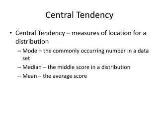
4. Central tendency • Central tendency = a measure of location or position of data, i.e. the ‘average’ • This basically means calculating things like: • Mean (arithmetic mean) • Median • Mode • Others • E.g. geometric mean (distn. skewed to the right), weighted mean • Nice table in Petrie and Sabin (Chapter 5) summarising advantages and disadvantages of all measurements

5. Central tendency – Mean, Median • Mean = Sum of your data/total number of measurements • Algebraically defined • Affected by skewed data THEREFORE good to use for normally distributed variables • Median = The midpoint of your values i.e. what the ‘halfway’ value in your data is • If the observations are arranged in increasing order, the median would be the middle value • Not algebraically defined • Not affected by skewed data THEREFORE good to use for non-normally distributed variables

6. Distributions Median Mean Mean and median the same

7. Central tendency - Mode • Mode = the value that occurs the most frequently in a data set • Generally means more if you have categorical data e.g. The most common litter size of bearded collie dogs is 7 • Not often used What is the mode?

8. Spread • Spread = measure of dispersion or variability (variation) of data • This basically means calculating things like: • Range • Percentiles (Quartiles, Interquartile range) • Variance • Standard deviation • Others • E.g. coefficient of variation • Nice table in Petrie and Sabin (Chapter 6) summarising main points about these measurements

9. Range and percentiles • Range = the range between the minimum and maximum values of your data • Gives an indication of spread at a very basic level • Distorted by outliers (get a large range) • Percentiles = if data is ordered from lowest to highest, these divide the data up into ‘compartments’ • E.g. The 5th percentile is the point alongthe data below which 5% of the data lies; the 20th percentile is the point in the data below which 20% of the data lies • Special types of percentiles are called ‘quartiles’ – these divide the data into 4 equal parts (the 25th, 50th and 75th percentiles) • From these, you get an ‘interquartile range’ - IQR, which is values between the 25th and 75th percentiles • The 50th percentile is the median • Not distorted by outliers

10. Range = 22-28 (6) Q1 (25th percentile) = 24 Q3 (75th percentile) = 26 IQR = 24-26 (2) Range = 0.12-134 (133.9) Q1 (25th percentile) = 6 Q3 (75th percentile) = 36 IQR = 6-36 (30) What conclusions can we draw about what to use when??

11. Rule of thumb • Mean and range = good to use for normally distributed variables • Median and interquartile range = good to use for non-normally distributed variables

12. Variance • Variance = the deviations of the data values from the mean • e.g. If the data are bunched around the mean, the variance is small; if the data are spread out, the variance is large • Calculated by squaring each distance between the observations and the mean • We then take the mean of this (add all values together and divide by the total number of observations minus 1) • DON’T WORRY ABOUT HOW TO DO THIS! This is what computers are for! • Measured in the same units as the observations, but squared e.g. If the units are grams, the variance will be in grams squared

13. Mean = 26 Variance = 430 Mean = 23 Variance = 11090

14. Example • If we had 6 observations (with mean = 0.17): 15, 18, -14, -17, -3 and 2 • What is the variance? = (15 – 0.17)2 + (18-0.17) 2 + (-14 – 0.17) 2 + (-17 – 0.17) 2 + (-3 – 0.17) 2 + (2-0.17) 2/6-1 = 209.37 It is n-1 to reduce bias (again don’t worry too much!)

15. Standard Deviation (SD) • Standard deviation = square root of the variance • The average of the deviations of the observations from the mean • Therefore the units are the same as for the observations – more convenient • If we have a normally distributed dataset, then the mean +/- 2 x standard deviations approximately encompasses the central 95% of observations

16. What about the standard error of the mean (SE or SEM)? • Similar to standard deviation, but relates to the precision of the sample mean as an estimate of the population mean • Can use SEM to construct confidence intervals • This will be covered in greater detail in another session

17. General rule • Standard deviation, variance and SEM are for normally distributed variables only • For non-normally distributed variables, stick with interquartile range

18. Equal variances? • It is an assumption of some of the tests used to compare different continuous data groups (e.g. T-tests, ANOVAs) that the variances must be equal (homogeneity of variance) in the groups compared • This is because these tests are not particularly robust under conditions of heterogeneity of variance • In order to use these tests, you need to know whether your groups meet these criteria – if they do not, you need to use other non-parametric tests, or transform your data to fit the assumptions

19. Tests for equal variances • Eyeball the distributions! • Levene’s test (two or more groups) • Null hypothesis – groups have equal variances • Calculation not affected by normality status • F-test (variance-ratio test; two groups only) • Calculation is affected by non-normal data • Bartlett’s test (two or more groups) • Calculation is affected by non-normal data

20. Next month • The bunfight that is: • P-values.................! • Type I and Type II errors