Introduction to Basic Statistical Methodology
Learn about random variation in population distributions, the importance of statistics in real issues, and hypothesis testing using practical examples. Explore how to analyze and interpret data effectively.

Introduction to Basic Statistical Methodology
E N D
Presentation Transcript
What is “random variation” in the distribution of a population? Examples: Toasting time, Temperature settings, etc.… POPULATION 1:Little to no variation (e.g., product manufacturing) In engineering situations such as this, we try to maintain “quality control”… i.e., “tight tolerance levels,” high precision, low variability. O OOOO But what about a population of, say, people?
What is “random variation” in the distribution of a population? Examples: Gender, Race, Age, Height, Drug Response (e.g., cholesterol level),… POPULATION 1:Little to no variation (e.g., product manufacturing) POPULATION 2:Little to no variation (e.g., clones) Most individual values ≈ population mean value Density NOT REALISTIC!!! Very little variation about the mean!
What is “random variation” in the distribution of a population? Examples: Gender, Race, Age, Height, Drug Response (e.g., cholesterol level),… POPULATION 2:Little to no variation (e.g., clones) POPULATION 3:Much variation (more realistic) Much more variation about the mean! Density
GLOBAL OPERATION DYNAMICS, INC. What are “statistics,” and how can they be applied to real issues? • Example: Suppose a certain company insists that it complies with “gender equality” regulations among its employee population, i.e., approx. 50% male and 50% female. To test this claim, let us select a random sample of n = 100 employees, and count X = the number of males. (If the claim is true, then we expect X 50.) etc. Sample size n partially depends on the power of the test, i.e., the desired probability of correctly rejecting a false null hypothesis ( 80%). The larger the n, the higher the power.
X = 64 males (+ 36 females) GLOBAL OPERATION DYNAMICS, INC. What are “statistics,” and how can they be applied to real issues? • Example: Suppose a certain company insists that it complies with “gender equality” regulations among its employee population, i.e., approx. 50% male and 50% female. To test this claim, let us select a random sample of n = 100 employees, and count X = the number of males. (If the claim is true, then we expect X 50.) etc. Questions: If the claim is true, how likely is this experimental result? (“p-value”) Could the difference (14 males) be due to random chance variation, or is it statistically significant?
...... …..from 0 to 100 Heads….. The experiment in this problem can be modeled by a random sequence of n = 100 independent coin tosses (Heads = Male, Tails = Female). It can be mathematically proved that, if the coin is “fair” (“unbiased”), then in 100 tosses: • probability of obtaining at least 0 Heads away from 50 is = 1.0000 “certainty” • probability of obtaining at least 1 Head away from 50 is = 0.9204 • probability of obtaining at least 2 Heads away from 50 is = 0.7644 • probability of obtaining at least 3 Heads away from 50 is = 0.6173 • probability of obtaining at least 4 Heads away from 50 is = 0.4841 • probability of obtaining at least 5 Heads away from 50 is = 0.3682 • probability of obtaining at least 6 Heads away from 50 is = 0.2713 • probability of obtaining at least 7 Heads away from 50 is = 0.1933 • probability of obtaining at least 8 Heads away from 50 is = 0.1332 • probability of obtaining at least 9 Heads away from 50 is = 0.0886 • probability of obtaining at least 10 Heads away from 50 is = 0.0569 • probability of obtaining at least 11 Heads away from 50 is = 0.0352 • probability of obtaining at least 12 Heads away from 50 is = 0.0210 • probability of obtaining at least 13 Heads away from 50 is = 0.0120 • probability of obtaining at least 14 Heads away from 50 is = 0.0066 etc. 0 The = .05 cutoff is called the significance level. 0.0066 is called the p-value of the sample. Because our p-value (.0066) is less than the significance level (.05), our data suggest that the coin is indeed biased, in favor of Heads. Likewise, our evidence suggests that employee gender in this company is biased, in favor of Males.
GLOBAL OPERATION DYNAMICS, INC. What are “statistics,” and how can they be applied to real issues? HYPOTHESIS EXPERIMENT • Example: Suppose a certain company insists that it complies with “gender equality” regulations among its employee population, i.e., approx. 50% male and 50% female. To test this claim, let us select a random sample of n = 100 employees, and count X = the number of males. (If the claim is true, then we expect X 50.) OBSERVATIONS X = 64 males (+ 36 females) etc. Questions: If the claim is true, how likely is this experimental result? (“p-value”) Could the difference (14 males) be due to random chance variation, or is it statistically significant?
...... The experiment in this problem can be modeled by a random sequence of n = 100 independent coin tosses (Heads = Male, Tails = Female). It can be mathematically proved that, if the coin is “fair” (“unbiased”), then in 100 tosses: • probability of obtaining at least 0 Heads away from 50 is = 1.0000 “certainty” • probability of obtaining at least 1 Head away from 50 is = 0.9204 • probability of obtaining at least 2 Heads away from 50 is = 0.7644 • probability of obtaining at least 3 Heads away from 50 is = 0.6173 • probability of obtaining at least 4 Heads away from 50 is = 0.4841 • probability of obtaining at least 5 Heads away from 50 is = 0.3682 • probability of obtaining at least 6 Heads away from 50 is = 0.2713 • probability of obtaining at least 7 Heads away from 50 is = 0.1933 • probability of obtaining at least 8 Heads away from 50 is = 0.1332 • probability of obtaining at least 9 Heads away from 50 is = 0.0886 • probability of obtaining at least 10 Heads away from 50 is = 0.0569 • probability of obtaining at least 11 Heads away from 50 is = 0.0352 • probability of obtaining at least 12 Heads away from 50 is = 0.0210 • probability of obtaining at least 13 Heads away from 50 is = 0.0120 • probability of obtaining at least 14 Heads away from 50 is = 0.0066 etc. 0 PROBABILITY The = .05 cutoff is called the significance level. THEORY ANALYSIS 0.0066 is called the p-value of the sample. Because our p-value (.0066) is less than the significance level (.05), our data suggest that the coin is indeed biased, in favor of Heads. Likewise, our evidence suggests that employee gender in this company is biased, in favor of Males. CONCLUSION
“Classical Scientific Method” • Hypothesis – Define the study population... What’s the question? • Experiment – Designed to test hypothesis • Observations – Collect sample measurements • Analysis – Do the data formally tend to support or refute the hypothesis, and with what strength? (Lots of juicy formulas...) • Conclusion – Reject or retain hypothesis; is the result statistically significant? • Interpretation – Translate findings in context! Statistics is implemented in each step of the classical scientific method!