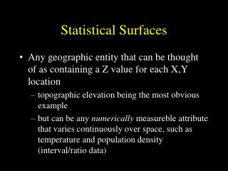

Statistical Surfaces
E N D
Presentation Transcript
Statistical Surfaces • Any geographic entity that can be thought of as containing a Z value for each X,Y location • topographic elevation being the most obvious example • but can be any numerically measureble attribute that varies continuously over space, such as temperature and population density (interval/ratio data)
Surfaces • Statistical surface • Continuous • Discrete
Statistical Surfaces • Two types of surfaces: • data are not countable (i.e. temperature) and geographic entity is conceptualized as a field • punctiform: data are composed of individuals whose distribution can be modeled as a field (population density)
2 2 3 2 2 3 3 6 3 3 3 4 4 2 2 3 4 4 3 1 2 2 3 2 1 Statistical Surfaces • Surface from punctiform data Point data Density surface Distribution of trees Find # of trees w/in the neighborhood of each grid cell
Statistical Surfaces • Storage of surface data in GIS • raster grid • TIN • isarithms (e.g. contours for topographic elevation) • lattice
Statistical Surfaces • Isarithm 10 20 30 40 50 80 70 60 60
Statistical Surfaces • Lattice: a set of points with associated Z values Regular Irregular
Statistical Surfaces • Interpolation • estimating the values of locations for which there is no data using the known data values of nearby locations • Extrapolation • estimating the values of locations outside the range of available data using the values of known data We will be talking about point interpolation
Statistical Surfaces Estimating a point here: interpolation Sample data
Statistical Surfaces Estimating a point here: interpolation Estimating a point here: extrapolation
Statistical Surfaces • Interpolation: Linear interpolation If A = 8 feet and B = 4 feet then C = (8 + 4) / 2 = 6 feet Sample elevation data A C B Elevation profile
Statistical Surfaces • Interpolation: Nonlinear interpolation Sample elevation data Often results in a more realistic interpolation but estimating missing data values is more complex A C B Elevation profile
Statistical Surfaces • Interpolation: Global • use all known sample points to estimate a value at an unsampled location Use entire data set to estimate value
Statistical Surfaces • Interpolation: Local • use a neighborhood of sample points to estimate a value at an unsampled location Use local neighborhood data to estimate value, i.e. closest n number of points, or within a given search radius
Statistical Surfaces • Interpolation: Distance Weighted (Inverse Distance Weighted - IDW) • the weight (influence) of a neighboring data value is inversely proportional to the square of its distance from the location of the estimated value 100 4 160 3 2 200
Statistical Surfaces • Interpolation: IDW Weights Adjusted Weights 1 / (42) = .0625 1 / (32) = .1111 1 / (22) = .2500 .0625 / .0625 = 1 .1111 / .0625 = 1.8 .2500 / .0625 = 4 100 x 1 = 100 160 x 1.8 = 288 200 x 4 = 800 100 100 +288 + 800 = 1188 4 1188 / 6.8 = 175 160 3 2 200
Statistical Surfaces • Interpolation: 1st degree Trend Surface • global method • multiple regression (predicting z elevation with x and y location • conceptually a plane of best fit passing through a cloud of sample data points • does not necessarily pass through each original sample data point
Statistical Surfaces • Interpolation: 1st degree Trend Surface In two dimensions In three dimensions z y y x x
Statistical Surfaces • Interpolation: Spline and higher degree trend surface • local • fits a mathematical function to a neighborhood of sample data points • a ‘curved’ surface • surface passes through all original sample data points
Statistical Surfaces • Interpolation: Spline and higher degree trend surface In two dimensions In three dimensions z y y x x
Statistical Surfaces • Interpolation: kriging • common for geologic applications • addresses both global variation (i.e. the drift or trend present in the entire sample data set) and local variation (over what distance do sample data points ‘influence’ one another) • provides a measure of error