Asymptotic Notations in Algorithm Analysis
200 likes | 710 Vues
Learn about the significance of asymptotic analysis and complexity notations in algorithm performance evaluation for large input sizes. Explore key concepts such as O, Θ, and Ω notation to compare growth rates effectively.

Asymptotic Notations in Algorithm Analysis
E N D
Presentation Transcript
Asymptotic Analysis CLRS, Sections 3.1 – 3.2
Asymptotic Complexity • Running time of an algorithm as a function of input size n, for large n. • Expressed using only the highest-order term in the expression for the exact running time. • Describes behavior of function in the limit. • Written using Asymptotic Notation. CS 321 - Data Structures
Asymptotic Notation • Q, O, W, o, w • Defined for functions over the natural numbers. • Ex:f(n) = Q(n2). • Describes how f(n) grows in comparison to n2. • Defines a set of functions; in practice used to compare growth rate of two functions. • The notations describe the relationship between the defining function and a defined set of functions. CS 321 - Data Structures
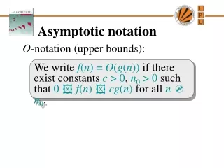
O-notation For function g(n), we define O(g(n)), big-O of n, as the set: O(g(n)) = {f(n) : positive constants c and n0,such that n n0,we have 0 f(n) cg(n) } Intuitively: Set of all functions whose rate of growth is the same as or lower than that of g(n). g(n) is an asymptotic upper bound for f(n). f(n) = (g(n)) f(n) = O(g(n)) (g(n)) O(g(n)) CS 321 - Data Structures
-notation For function g(n), we define (g(n)), big-Omega of n, as the set: (g(n)) = {f(n) : positive constants c and n0,such that n n0, we have 0 cg(n) f(n)} Intuitively: Set of all functions whose rate of growth is the same as or higher than that of g(n). g(n) is an asymptotic lower bound for f(n). f(n) = (g(n)) f(n) = (g(n)) (g(n)) (g(n)) CS 321 - Data Structures
-notation For function g(n), we define (g(n)), big-Theta of n, as the set: (g(n)) ={f(n) : positive constants c1, c2, and n0, such that n n0,we have 0 c1g(n) f(n) c2g(n)} Intuitively: Set of all functions that have the same rate of growth as g(n). g(n) is an asymptotically tight bound for f(n). CS 321 - Data Structures
Relationship Between Q, O, W CS 321 - Data Structures
Relationship Between Q, W, O • (g(n)) = O(g(n)) ÇW(g(n)) • In practice, asymptotically tight bounds are obtained from asymptotic upper and lower bounds. Theorem : For any two functions g(n) and f(n), f(n) = (g(n))iff f(n) =O(g(n)) and f(n) = (g(n)). CS 321 - Data Structures
o-notation g(n) is anupper bound for f(n)that is not asymptotically tight. For a given function g(n), the set little-o: o(g(n))= {f(n): c > 0, n0 > 0 such that n n0, we have0 f(n)<cg(n)}. Intuitively: Set of all functions whose rate of growth is lower than that of g(n). CS 321 - Data Structures
w-notation g(n) is alower bound for f(n)that is not asymptotically tight. For a given function g(n), the set little-omega: w(g(n))= {f(n): c > 0, n0 > 0 such that n n0, we have0 cg(n) < f(n)}. Intuitively: Set of all functions whose rate of growth is higher than that of g(n). CS 321 - Data Structures
Comparison of Functions f g ~a b f (n) = O(g(n))~ a b f (n) = (g(n))~ a b f (n) = (g(n))~ a = b f (n) = o(g(n))~ a < b f (n) = w(g(n))~ a > b CS 321 - Data Structures
Limit Definitions of Asymptotic Notations • o-notation (little-o): • f(n) becomes insignificant relative to g(n)as n approaches infinity: lim[f(n) / g(n)] = 0 n • w-notation (little-omega): • f(n) becomes arbitrarily large relative to g(n)as n approaches infinity: lim[f(n) / g(n)] = n CS 321 - Data Structures
Limit Definitions of Asymptotic Notations • -notation (Big-theta): • f(n) relative to g(n)equals a constant, c, which is greater than 0 and less than infinity as n approaches infinity: 0 < lim[f(n) / g(n)] < n CS 321 - Data Structures
Limit Definitions of Asymptotic Notations • O-notation (Big-o): • f(n)ÎO(g(n)) Þf(n)Î(g(n))and f(n)Îo(g(n)) • f(n) relative to g(n)equals some value less than infinity as n approaches infinity: lim[f(n) / g(n)] < n • -notation (Big-omega): • f(n)Î (g(n)) Þf(n)Î(g(n))and f(n)Îw(g(n)) • f(n) relative to g(n)equals some value greater than 0 as n approaches infinity: 0 <lim[f(n) / g(n)] n CS 321 - Data Structures
Examples Use limit definitions to prove: • 10n -3n O(n2) • 3n4 (n3) • n2/2 - 3n Q(n2) • 22n Q(2n) CS 321 - Data Structures
Examples Use limit definitions to prove: • 10n -3n O(n2) – Yes! lim[ 10n -3n / n2 ] = 0 n • 3n4 (n3) – Yes! lim[ 3n4 / n3 ] = n • n2/2 - 3n Q(n2) – Yes! lim[ n2/2 - 3n/ n2 ] = 1/2 n • 22n Q(2n) – No! lim[ 22n / 2n ] = n CS 321 - Data Structures
Why Do We Care? CS 321 - Data Structures
Complexity and Tractability Assuming the microprocessor performs 1 billion ops/s. CS 321 - Data Structures