Download

1 / 39
390 likes | 572 Vues
Pricing and Evaluating a Bond Portfolio Using a Regime-Switching Markov Model. Leela Mitra* Rogemar Mamon Gautam Mitra Centre for the Analysis of Risk and Optimisation Modelling. *sponsored by EPSRC and OptiRisk. Outline. 1. Motivation & insights 2. Problem setting 3. Novel features

E N D
Pricing and Evaluating a Bond Portfolio Using a Regime-Switching Markov Model Leela Mitra* Rogemar Mamon Gautam Mitra Centre for the Analysis of Risk and Optimisation Modelling *sponsored by EPSRC and OptiRisk
Outline 1. Motivation & insights 2. Problem setting 3. Novel features 4. Asset model 5. Computational study
1. Motivation & Insights • Credit risk – risk that a counterparty’s creditworthiness changes, in particular that of default on financial obligations. • An important consideration for investors. • An important distinction Rogers (1999) notes “the first and most important thing to realise about modelling credit risk is that we may be trying to answer questions of two different types”; Pricing credit risky assets and quantifying their risk exposure. • Appropriate integration of significant risks. - Market risk in particular, interest rate risk. - Credit risk.
1. Motivation & Insights • Two main categories credit risk model - Structural models. Merton (1974), Option theoretic, Debt contingent claim on firm’s assets. - Reduced form models. Jump processes.
2. Problem Setting - Jarrow, Lando & Turnbull (1997) (JLT) • Credit migration process described by Markov chain. • Fractional recovery on default; ηof par value. • Interest rate process. - Any process can be used to represent the default-free rate. • Connecting risk neutral measure, P with physical world measure, leading to… • Arbitrage-free pricing. - Prices of defaultable bonds are the expected values under P, discounted at the default-free rate.
2. Problem Setting - Thomas, Allen & Morkel-Kingsbury (2002) • Adapt JLT framework. • Markov chain which represents the economy; “Regime-switching model”. • Price defaultable bonds.
3. Problem Setting – Our Work • Pricing. • - Price a portfolio of defaultable bonds. • - Similar model to Thomas et al. • Risk quantification. • - Extend the model to the physical measure to simulate the bond portfolio value. • - Calculate Value at Risk (VaR) and Conditional Value at Risk (CVaR) one year ahead.
3. Novel Features • Yield Curve Modelling; no arbitrage across interest rates. • Bond stripping: Discovering of yield and credit spreads using quadratic programming (QP1), • - constraints remove price anomalies. • Calibration of the risk neutral credit migration process using quadratic programming (QP2), • - constraints remove negative probabilities.
4. Asset Model Economy Process CtE 0 - Treasury 1 – Highest rated bonds M-1 Worst rated bonds M Default - absorbing state. Rating Migration Process CtR Interest Rate Process CtI
4. Asset Models – Interest Rate Process • Thomas et al. model spot rate without restrictions, on process for arbitrage. • Whole yield curve should be modelled, – Heath, Jarrow & Morton (1992). • Interest Rates are functions of two time dimensions, - current time t, - time to maturity T.
4. Asset Models – Interest Rate Process • Model an auxiliary binomial process to describe underlying interest rate process. S0 ={0} S1 ={u, d} S2 ={uu, ud, du, dd} S3 ={uuu, …} Figure 1: Possible evolution of state space tree over t = {0,1,2,3}
4. Asset Models – Interest Rate Process • Forward Rate Process
4. Asset Models – Interest Rate Process • Treasury zero coupon bond prices process and forward rate process are equivalent. • Zero coupon bond price process • Absence of arbitrage can be understood as
4. Asset Models – Interest Rate Process • Continuously compounding forward rate • Continuous time process described by SDE • Defining, the discrete process converges to the continuous.
4. Asset Models – Interest Rate Process • Assuming • No arbitrage condition becomes • Drift of process under the risk neutral measure is well defined, given the observed volatility.
4. Asset Models – Risky bond price • The price of a credit risky bond is, discounted expected value under the risk neutral measure, where,
5. Computational Study • Part 1 – Bond stripping; Discovering of yield and credit spreads. • Part 2 – Model calibration. • Part 3 – Simulation of bond portfolio value so determining its distribution.
5. Computational Study Bond Stripping - Motivation • Bonds priced using zero coupon bond prices. - Any bond’s price is determined using zero coupon bonds prices as discount factors. - Models for term structure describe zero coupon bond prices. • Market Data Available. - Mainly coupon bonds available in market. - Model calibration involves stripping coupons from coupon bonds to derive underlying zero coupon bond prices. • Jarrow et al. - Bucket bonds by rating and maturity and find average prices and coupons for each bucket. - Solve system triangular equations to get zero coupon prices. - Can lead to mispricing.
5. Computational Study Bond Stripping - Motivation • Allen, Thomas and Zheng - Use linear programming to find zero coupon bond prices. - Minimise absolute pricing errors. - Constraints are used to remove anomalies =>mispricing. • Our Work - Use same formulation but with quadratic programming so minimising squared pricing errors. - Equivalent to constrained regression.
5. Computational Study Bond Stripping - Formulation • Credit ratings {0, 1,…, M-1} • Time set { 0,…,T} • N coupon bonds - where bond b, 1 b N, - current market price vb , - rating r(b), - pays cash flow cb(t) at time t. • Zero coupon bond prices - zk(t) price of a zero coupon bond, with rating k, which pays 1 at time t.
5. Computational Study Bond Stripping - Formulation for bond b let ob be the pricing error ‘over’ let ub be the pricing error ‘under’ Minimise b (ob +ub ) 2 (1) subject to vb + ob = t cb(t) zr(b)(t) + ub b {1,…,N} (2) z 0(t) z 0(t+1) (1+ m(t)) t {0,…,T} (3) z k(t+1) - z k+1(t+1) z k(t) - z k+1(t) t {0,…,T} k {0,…,M-1} (4) m(t) – minimum discount rate over (t,t+1].
5. Computational Study Bond Stripping – Allowing Mispricing • If we adapt (4) we allow some types of mispricing of zero coupon bonds. • Minimise b (ob +ub ) 2 (1) subject to vb + ob = t cb(t) zr(b)(t) + ub b {1,…,N} (2) z 0(t) z 0(t+1) (1+ m(t)) t {0,…,T} k {0,…,M-1} (3) z 0(t+1) - z k+1(t+1) z 0(t) - z k+1(t) t {0,…,T} k {0,…,M-1} (4)
5. Computational Study - Model Calibration • Each chain • -Determine relevant states. • Determine physical world and risk neutral measures. • Economy • Classify years as good or bad, using observed transitions to lower ratings and default. • Physical probabilities as observed frequencies of transitions. • Risk neutral measure assumed to be same as real world.
5. Computational Study - Model Calibration • Interest Rate Process • From observations of daily yield curve, • we derive observations of volatility. • - Fit to functional form, • to give our volatility function. Vasicek model. • - Risk neutral drift is then well defined by no arbitrage condition.
5. Computational Study - Model Calibration • Interest Rate Process • The states of the processes are known, given • Forward rates/ zero coupon bonds processes. • Risk neutral probabilities are ½ by construction. • Physical probabilities are derived from the observed drift of the yield curve.
5. Computational Study – Model Calibration • Credit Rating Migrations • States are well defined; ratings classes and default state. • - Historical Standard & Poors default frequency data for physical world measure. • - Risk neutral measure backed out from zero coupon bond prices.
5. Computational Study – Model Calibration • Credit Rating Migrations - physical world measure - risk neutral / pricing measure - Similar expressions for when the economy is in state B
5. Computational Study – Model Calibration Credit Rating Migrations • Assuming the economy does not change, pricing equation is • . • So given the zero coupon bond prices we are able to derive the implied probabilities of default under the risk neutral measure, • , that is risk neutral probabilities over (0, T] are known.
5. Computational Study – Model Calibration Credit Rating Migrations • Risk neutral probabilities over (0, T0] can be found from zero coupon bond prices for bond maturing at time T0. • Risk neutral probabilities over (0, Tn] can be found from zero coupon bond prices for bond maturing at time Tn . • As process is Markov, if probabilities over (0, T n -1] and probabilities over (0, T n] are known we can derive probabilities over (T n -1, T n]. • We are able to derive risk neutral probabilities over all timeperiods, recursively.
5. Computational Study – Model Calibration Credit Rating Migrations • Negative values for the probabilities possible. • Nothing in structure of recursive equations solved that ensure probabilities take sensible values. • Solve set of recursive QPs with restrictions on values of probabilities. • - Initial Credit Fit – derives probabilities over (0,T0] given zero coupon bond prices maturing at T0 • - Recursive Credit Fit – derives probabilities over (Tn-1,Tn], • given zero coupon bond prices maturing at Tn and probabilities over (0,Tn-1] • Use prices at more than one date. • - Incorporates more information into risk neutral measure that is derived.
5. Computational Study – Model Calibration • Initial Credit Fit – derives probabilities over (0,T0]
5. Computational Study – Model Calibration • Recursive Credit Fit – derives probabilities over (Tn-1,Tn]
5. Computational Study- Simulation of VaR & CVaR
5. Computational Study- Simulation of VaR & CVaR
5. QP vs LP Efficient Frontier • Allen, Thomas and Zheng – LP Formulation • - Objective: Minimise b (ob +ub )