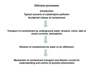
Regularization on graphs with function-adapted diffusion processes
Regularization on graphs with function-adapted diffusion processes. By A. D. Szlam, M. Maggioni, R. Coifman Presented by Eric Wang. 8-16-2007. Introduction and Motivation Setup and Notation Denoising and Regularization by Diffusion Application 1: Denoising of images


Regularization on graphs with function-adapted diffusion processes
E N D
Presentation Transcript
Regularization on graphs with function-adapted diffusion processes By A. D. Szlam, M. Maggioni, R. Coifman Presented by Eric Wang 8-16-2007
Introduction and Motivation • Setup and Notation • Denoising and Regularization by Diffusion Application 1: Denoising of images • Application 2: Graph Transductive Learning • Conclusion
Introduction/Motivation • Goal: Use graph diffusion techniques to approximate and study functions on a particular data set. • The use of graph diffusion is helpful in this case because it intrinsically reduces noise in data, i.e. the noise is contained (mostly) in the high frequency components. • An important contribution of this paper is that it uses the function of the data as well as the geometry of the data.
Setup/Notation Consider a finite weighted graph Consider , then we can define a natural filter acting on functions in V as We can consider K as a natural filter, then is a K step diffusion on the function f.
Setup/Notation We can define the weight matrix W as below Commonly We can set the parameter , which governs the random walk distance of the kernel, either globally, or have it vary locally. Zelnik-Manor and Perona proposed a self-tuning matrix using the following scheme: Here, a number m is fixed, and the distances at each point are scaled so that the m-th neighbor has distance 1. This method also truncated at the k-th nearest neighbor A global corresponds to a location dependent choice of in the standard exponential weights.
Setup/Notation Consider the eigenfunctions of K satisfying Any function can be written as since is an orthonormal basis. The index i indicates how oscillatory the function is. The higher i is, the more oscillatory, since measures the frequency of . We can measure smoothness by first defining the graph Laplacian Then the Sobolev norm measures smoothness where
Setup/Notation Several things of note: Projecting a function onto the first few terms of its expansion is by itself a smoothing operation, as the subspace spanned by the high frequency are the ones with a higher Sobolev norm. If f does not have uniform smoothness everywhere, then approximation by eigenfunctions is poor in the areas of lesser smoothness, and also spills over into the areas of greater smoothness
Denoising and Regularization by Diffusion A basic task is to denoise, i.e. regularize, a function f on a data set X. X is given, and is measured, where and is stochastic noise. The goal is to yield a function which approximates the unknown function f. If f is assumed to be smooth, then this implies that decays rapidly with i. Thus we can let
Data and Function-adapted Kernels To encourage averaging along “level sets” i.e. relatively smooth areas of f, one could let Or more generally Where is a setof features associated with f, evaluated at point x is a metric on the data set is a metric on the set of features The associated averaging kernel can then be used for denoising and learning. Such a kernel is called a function-adapted kernel. If then K will average locally, but much more along level sets of f than across them.
Application 1: Denoising Images 1.) Construct a graph G associated with image I. a.) d filters This method is extremely flexible, one could define our filters to be anything, wavelets or curvelets at different scales, edge filters, or patches of texture, or some measure of local statistics. b.) The graph G(I) will have vertices given by with weighted edges 2.) Compute the associated I-adapted diffusion operator . 3.) Let . Note here that the amount of denoising is governed by t, controls the amount the spatial coordinates are considered, and is a denoised version ofI.
Application 1: Denoising Images Examples showing some locations highlighted. The center top figure shows where t=1, and the right figure is t=2. Bottom figure shows examples of the 2-D Gaussian kernel
Results: Denoising Images A A is the original image f with noise N(0,.0244), B is the image using a 7x7 NL means patch graph. The W matrix is constructed as where each pixel studies its relation its 81 closest neighbors. One can balance between smoothing and fidelity to the original noisy image by B Where is a set parameter which is directly related to greater fidelity to the original image. To obtain image B, = .07, and K was iterated 3 times.
Results: Denoising Images C Image C shows the results from summing 9 curvelet denoisings, obtained by shifting the noisy image A either 1, 2, or 4 pixels in the vertical and/or horizontal directions, using only coefficients larger than . Image D shows the results from embedding the 9 curvelet denoisings in as coordinates. W was constructed D Then is constucted and applied ten times on the noisy image using where, = .1
Application II: Graph Transductive learning Here, one is given a few “labeled” examples And a large number of “unlabeled” examples The goal is to estimate the conditional distributions associated with each available examplex (labeled or unlabeled) by extending the labels to a function F dedined on the whole X. This is practical because the points in , while unlabeled, still give information relating to the geometry of the space. Using simple geometric smoothing works only if the structure of the classes is very simple with respect to the geometry of the data set. However, if the classes have additional structure on top of the underlying data set, this will not be preserved by smoothing geometrically. The solution would be to let the smoothing flow faster along the “edges” of class functions than across them.
Application II: Graph Transductive learning Let be the ith class, and let be 1 on the labeled points in the ith class, -1 on the labeled points of classes not equal to i, and 0 elsewhere. 1.) Construct a graph G associated X. W is computed only on the spatial coordinates of X 2.) Compute the associated diffusion operator 3.) Compute guesses at the soft class functions by regularizing , i.e. For multi-class problems, set
Application II: Graph Transductive learning Recall Then we can set where controls the and trade-off between the importance of the geometry of X and that of the set of estimates 4.) Construct a new G’ with function adapted diffusion kernel K’. 5.) Find C(x) by diffusing with K’, and finding
Results: Graph Transductive learning This was tested on the first 10,000 images MNIST handwriting data and Chapelle et al. 100 points were chosen as labeled, and all data was reduced to dimensionality 50. W was constructed as before, and the following smoothing algorithms were applied: Harmonic Classifier (HC) Same as Kernel Smoothing, except class labels are relabeled to 1 after each iteration Eigenfunction embedding (EF) See above for details, essentially, Kernel Smoothing (KS) See above. Function Adapted Harmonic Classifier (FAHC), Function Adapted Eigenfunction Embedding (FAEF) Function Adapted Kernel Smoothing (FAKS)
Results: Graph Transductive learning Comparison of the Various Methods of Diffusion smoothing Comparison of the Various Methods of Diffusion Smoothing versus the ones considered in Chapelle et al.
Conclusion Function-adapted smoothing is a very flexible process that lends itself well to image denoising and graph transductive learning and classification. These two problems are traditionally considered very different, but they can be tackled effectively using this framework, This presents a powerful approach to tackling a wide variety of problems by leveraging not only the data itself, but the intrinsic geometric distribution of the data. + = CRAZY DELICIOUS!!!