2.4 Base Excitation
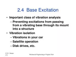
2.4 Base Excitation. Important class of vibration analysis Preventing excitations from passing from a vibrating base through its mount into a structure Vibration isolation Vibrations in your car Satellite operation Disk drives, etc. m. m. FBD of SDOF Base Excitation. System Sketch .

2.4 Base Excitation
E N D
Presentation Transcript
2.4 Base Excitation • Important class of vibration analysis • Preventing excitations from passing from a vibrating base through its mount into a structure • Vibration isolation • Vibrations in your car • Satellite operation • Disk drives, etc. Mechanical Engineering at Virginia Tech
m m FBD of SDOF Base Excitation System Sketch System FBD x(t) k c y(t) base Mechanical Engineering at Virginia Tech
SDOF Base Excitation (cont) For a car, The steady-state solution is just the superposition of the two individual particular solutions (system is linear). Mechanical Engineering at Virginia Tech
Particular Solution (sine term) With a sine for the forcing function, Use rectangular form to make it easier to add the cos term Mechanical Engineering at Virginia Tech
Particular Solution (cos term) With a cosine for the forcing function, we showed Mechanical Engineering at Virginia Tech
Magnitude X/Y Now add the sin and cos terms to get the magnitude of the full particular solution Mechanical Engineering at Virginia Tech
40 z =0.01 z =0.1 30 z =0.3 z =0.7 20 X/Y (dB) 10 0 -10 -20 0 0.5 1 1.5 2 2.5 3 Frequency ratio r The relative magnitude plot of X/Y versus frequency ratio: Called the Displacement Transmissibility Figure 2.13 Mechanical Engineering at Virginia Tech
From the plot of relative Displacement Transmissibility observe that: • X/Y is called Displacement Transmissibility Ratio • Potentially severe amplification at resonance • Attenuation for r > sqrt(2) Isolation Zone • If r< sqrt(2) transmissibility decreases with damping ratio Amplification Zone • If r >> 1 then transmissibility increases with damping ratio Xp~2Yz/r Mechanical Engineering at Virginia Tech
m Next examine the Force Transmitted to the mass as a function of the frequency ratio From FBD x(t) FT k c y(t) base Mechanical Engineering at Virginia Tech
40 z =0.01 z =0.1 30 z =0.3 z =0.7 20 F/kY (dB) 10 0 -10 -20 0 0.5 1 1.5 2 2.5 3 Frequency ratio r Plot of Force Transmissibility (in dB) versus frequency ratio Figure 2.14 Mechanical Engineering at Virginia Tech
Figure 2.15 Comparison between force and displacement transmissibility Force Transmissibility Displacement Transmissibility Mechanical Engineering at Virginia Tech
Example 2.4.1: Effect of speed on the amplitude of car vibration Mechanical Engineering at Virginia Tech
Model the road as a sinusoidal input to base motion of the car model Approximation of road surface: From the data give, determine the frequency and damping ratio of the car suspension: Mechanical Engineering at Virginia Tech
From the input frequency, input amplitude, natural frequency and damping ratio use equation (2.70) to compute the amplitude of the response: What happens as the car goes faster? See Table 2.1. Mechanical Engineering at Virginia Tech
Example 2.4.2: Compute the force transmitted to a machine through base motion at resonance From (2.77) at r =1: From given m, c, and k: From measured excitation Y = 0.001 m: Mechanical Engineering at Virginia Tech
2.5 Rotating Unbalance • Gyros • Cryo-coolers • Tires • Washing machines m0 e Machine of total mass m i.e. m0 included in m t e = eccentricitymo = mass unbalancew = rotation frequency k c Mechanical Engineering at Virginia Tech
Rx m0 w e q Ry Rotating Unbalance (cont) What force is imparted on the structure? Note it rotates with x component: From sophomore dynamics, Mechanical Engineering at Virginia Tech
Rotating Unbalance (cont) The problem is now just like any other SDOF system with a harmonic excitation m0ew2sin(wt) x(t) m k Note the influences on the forcing function (we are assuming that the mass m is held in place in the y direction as indicated in Figure 2.18) c Mechanical Engineering at Virginia Tech
Rotating Unbalance (cont) • Just another SDOF oscillator with a harmonic forcing function • Expressed in terms of frequency ratio r Mechanical Engineering at Virginia Tech
Figure 2.20: Displacement magnitude vs frequency caused by rotating unbalance Mechanical Engineering at Virginia Tech
Example 2.5.1:Given the deflection at resonance (0.1m), = 0.05 and a 10% out of balance, compute e and the amount of added mass needed to reduce the maximum amplitude to 0.01 m. At resonance r = 1 and Now to compute the added mass, again at resonance; Use this to find m so that X is 0.01: Here m0 is 10%m or 0.1m Mechanical Engineering at Virginia Tech
Example 2.5.2 Helicopter rotor unbalance Given Fig 2.21 Fig 2.22 Compute the deflection at 1500 rpm and find the rotor speed at which the deflection is maximum Mechanical Engineering at Virginia Tech
Example 2.5.2 Solution The rotating mass is 20 + 0.5 or 20.5. The stiffness is provided by the Tail section and the corresponding mass is that determined in Example 1.4.4. So the system natural frequency is The frequency of rotation is Mechanical Engineering at Virginia Tech
Now compute the deflection at r = 3.16 and =0.01 using eq (2.84) At around r = 1, the max deflection occurs: At r = 1: Mechanical Engineering at Virginia Tech
2.6 Measurement Devices • A basic transducer used in vibration measurement is the accelerometer. • This device can be modeled using the base equations developed in the previous section Here, y(t) is the measured response of the structure Mechanical Engineering at Virginia Tech
Base motion applied to measurement devices Accelerometer These equations should be familiar from base motion. Here they describe measurement! Strain Gauge Mechanical Engineering at Virginia Tech
Magnitude and sensitivity plots for accelerometers. Effect of damping on proportionality constant Fig 2.27 Fig 2.26 Magnitude plot showing Regions of measurement In the accel region, output voltage is nearly proportional to displacement Mechanical Engineering at Virginia Tech
2.7 Other forms of damping These various other forms of damping are all nonlinear. They can be compared to linear damping by the method of “equivalent viscous damping” discussed next. A numerical treatment of the exact response is given in section 2.9. Mechanical Engineering at Virginia Tech
The method of equivalent viscous damping:consists of comparing the energy dissipated during one cycle of forced response Assume a stead state resulting from a harmonic input and compute the energy dissipated per one cycle The energy per cycle for a viscously damped system is (2.101) Mechanical Engineering at Virginia Tech
Next compute the energy dissipated per cycle for Coulomb damping: Here we let u = t and du =dt and split up the integral according to the sign changes in velocity. Next compare this energy to that of a viscous system: (2.105) This yields a linear viscous system dissipating the same amount of energy per cycle. Mechanical Engineering at Virginia Tech
Using the equivalent viscous damping calculations, each of the systems in Table 2.2 can be approximated by a linear viscous system In particular, ceq can be used to derive amplitude expressions. However, as indicated in Section 2.8 and 2.9 the response can be simulated numerically to provide more accurate magnitude and response information. Mechanical Engineering at Virginia Tech
Hysteresis: an important concept characterizing damping • A plot of displacement versus spring/damping force for viscous damping yields a loop • At the bottom is a stress strain plot for a system with material damping of the hysteretic type • The enclosed area is equal to the energy lost per cycle Mechanical Engineering at Virginia Tech
The measured area yields the energy dissipated. For some materials, called hysteretic this is Here the constant , a measured quantity is called the hysteretic damping constant, k is the stiffness and X is the amplitude. Comparing this to the viscous energy yields: Mechanical Engineering at Virginia Tech
Hysteresis gives rise to the concept of complex stiffness Substitution of the equivalent damping coefficient and using the complex exponential to describe a harmonic input yields: Mechanical Engineering at Virginia Tech
2.8 Numerical Simulation and Design • Four things we can do computationally to help solve, understand and design vibration problems subject to harmonic excitation • Symbolic manipulation • Plotting of the time response • Solution and plotting of the time response • Plotting magnitude and phase Mechanical Engineering at Virginia Tech
Symbolic Manipulation Let and What is This can be solved using Matlab, Mathcad or Mathematica Mechanical Engineering at Virginia Tech
Symbolic Manipulation Solve equations (2.34) using Mathcad symbolics : Enter this Choose evaluate under symbolics to get this Mechanical Engineering at Virginia Tech
In MATLAB Command Window >> syms z wn w f0 >> A=[wn^2-w^2 2*z*wn*w;-2*z*wn*w wn^2-w^2]; >> x=[f0 ;0]; >> An=inv(A)*x An = [ (wn^2-w^2)/(wn^4-2*wn^2*w^2+w^4+4*z^2*wn^2*w^2)*f0] [ 2*z*wn*w/(wn^4-2*wn^2*w^2+w^4+4*z^2*wn^2*w^2)*f0] >> pretty(An) [ 2 2 ] [ (wn - w ) f0 ] [ --------------------------------- ] [ 4 2 2 4 2 2 2 ] [ wn - 2 wn w + w + 4 z wn w ] [ ] [ z wn w f0 ] [2 ---------------------------------] [ 4 2 2 4 2 2 2] [ wn - 2 wn w + w + 4 z wn w ] Mechanical Engineering at Virginia Tech
40 z =0.01 Design value 30 z =0.05 z =0.1 20 z =0.2 z =0.5 X/Y (dB) 10 0 -10 -20 0 0.5 1 1.5 2 2.5 3 Frequency ratio r Magnitude plots: Base Excitation %m-file to plot base excitation to mass vibration r=linspace(0,3,500); ze=[0.01;0.05;0.1;0.20;0.50]; X=sqrt( ((2*ze*r).^2+1) ./ ( (ones(size(ze))*(1-r.*r).^2) + (2*ze*r).^2) ); figure(1) plot(r,20*log10(X)) The values of z can then be chosen directly off of the plot. For Example: If the T.R. needs to be less than 2 (or 6dB) and r is close to 1 then z must be more than 0.2 (probably about 0.3). Mechanical Engineering at Virginia Tech
40 z =0.01 30 z =0.05 z =0.1 20 z =0.2 z =0.5 FT /kY (dB) 10 0 -10 -20 0 0.5 1 1.5 2 2.5 3 Frequency ratio r Force Magnitude plots: Base Excitation %m-file to plot base excitation to mass vibration r=linspace(0,3,500); ze=[0.01;0.05;0.1;0.20;0.50]; X=sqrt( ((2*ze*r).^2+1) ./ ( (ones(size(ze))*(1-r.*r).^2) + (2*ze*r).^2) ); F=X.*(ones(length(ze),1)*r).^2; figure(1) plot(r,20*log10(F)) Mechanical Engineering at Virginia Tech
Numerical Simulation We can put the forced case: Into a state space form Mechanical Engineering at Virginia Tech
Numerical Integration Zero initial conditions Using the ODE45 function >>TSPAN=[0 10]; >>Y0=[0;0]; >>[t,y] =ode45('num_for',TSPAN,Y0); >>plot(t,y(:,1)) 5 4 3 2 Including forcing 1 function Xdot=num_for(t,X) m=100;k=1000;c=25; ze=c/(2*sqrt(k*m)); wn=sqrt(k/m); w=2.5;F=1000;f=F/m; f=[0 ;f*cos(w*t)]; A=[0 1;-wn*wn -2*ze*wn]; Xdot=A*X+f; 0 Displacement (m) -1 -2 -3 -4 -5 0 2 4 6 8 10 Time (sec) Mechanical Engineering at Virginia Tech
Example 2.8.2: Design damping for an electronics model • 100 kg mass, subject to 150cos(5t) N • Stiffness k=500 N/m, c = 10kg/s • Usually x0=0.01 m, v0 = 0.5 m/s • Find a new c such that the max transient value is 0.2 m. Mechanical Engineering at Virginia Tech
Response of the board is; transient exceeds design specification value 0.4 0.2 0 Displacement (m) -0.2 -0.4 0 10 20 30 40 Time (sec) Mechanical Engineering at Virginia Tech
To run this use the following file: function Xdot=num_for(t,X) m=100;k=500;c=10; ze=c/(2*sqrt(k*m)); wn=sqrt(k/m); w=5;F=150;f=F/m; f=[0 ;f*cos(w*t)]; A=[0 1;-wn*wn -2*ze*wn]; Xdot=A*X+f; Create function to model forcing >>TSPAN=[0 40]; >> Y0=[0.01;0.5]; >>[t,y] = ode45('num_for',TSPAN,Y0); >> plot(t,y(:,1)) >> xlabel('Time (sec)') >> ylabel('Displacement (m)') >> grid Matlab command window Rerun this code, increasing c each time until a response that satisfies the design limits results. Mechanical Engineering at Virginia Tech
Solution: code it, plot it and change c until the desired response bound is obtained. 0.3 Meets amplitude limit when c=195kg/s 0.2 0.1 Displacement (m) 0 -0.1 0 10 20 30 40 Time (sec) Mechanical Engineering at Virginia Tech
2.9 Nonlinear Response Properties • More than one equilibrium • Steady state depends on initial conditions • Period depends on I.C. and amplitude • Sub and super harmonic resonance • No superposition • Harmonic input resulting in nonperiodic motion • Jumps appear in response amplitude Mechanical Engineering at Virginia Tech
Computing the forced response of a non-linear system A non-linear system has a equation of motion given by: Put this expression into state-space form: In vector form: Mechanical Engineering at Virginia Tech
Numerical form Vector of nonlinear dynamics Input force vector Euler equation is Mechanical Engineering at Virginia Tech
Cubic nonlinear spring (2.9.1) 2 1 0 Displacement (m) -1 Non-linearity included Linear system -2 0 2 4 6 8 10 Time (sec) Superharmonic resonance Mechanical Engineering at Virginia Tech