Environmental Modeling Basic GIS Functions for Suitability Index Modeling
Environmental Modeling Basic GIS Functions for Suitability Index Modeling. GIS Functions for Suitability Index. Overlay and buffer The fundamental difference between GIS and other computer mapping. courtesy: Mary Ruvane, http://ils.unc.edu/. Vector Raster. 3. Overlay.

Environmental Modeling Basic GIS Functions for Suitability Index Modeling
E N D
Presentation Transcript
Environmental Modeling Basic GIS Functions forSuitability Index Modeling
GIS Functions for Suitability Index • Overlay and buffer • The fundamental difference between GIS and other computer mapping
courtesy: Mary Ruvane, http://ils.unc.edu/ VectorRaster
3. Overlay Union, Intersect, and Identity Clip, Erase, and Update
Logic Overlay • Finding areas where certain conditions occur • Boolean logic Mary Ruvane, UNC –Chapel Hill
Union OUT INPUT Feature UNION Feature # # ATTRIBUTE # ATT 1 1 0 1 0 2 1 0 2 102 3 2 A 1 4 2 A 2 102 5 3 B 2 102 6 3 B 1 7 2 A 3 103 8 3 B 3 103 9 4 C 3 103 10 5 D 3 103 11 4 C 1 12 4 C 2 102 13 5 D 2 102 14 5 D 1 15 1 2 102 INPUT Feature UNION Feature # ATTRIBUTE # ATTRIBUTE 1 0 1 0 2 A 2 102 3 B 3 103 4 C 5 D
Intersect and Identity • Intersect • Identity
Intersect OUT PopElev PopRank PopWeight PopW*R EleRank EleWeight EleW*R Sum # # ATT# ATT 1 11 2 2 H 2 100 3 3 M2 100 4 2 H 3 150 5 3 M3 150 6 4 L 3 150 7 5 S3 150 8 4 L2 100 9 5 S 2 100
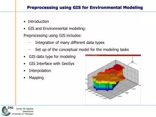
4. Approximation Buffer and Buffer Region Near and Point Distance
GRID Functions - Spatial Analyst Distance, Density, Surface Analysis, Cell Statistics, Neighborhood Statistics, Zonal Statistics
Cumulative Travel Cost Start Point Data Layer Friction Surface Data Layer Cumulative Travel Time Data Layer
Cost Weighted Distance DEM Friction surface Cost weighted distance S. Fritz and S. Carver GIS/EM4 2000
Athens Sounion
Least-Cost Analysis: Path 1 Path 1 with topography (above) and archaeologically-known sites (left).The background (left) is the cost layer—the darker color = higher costDistance: about 69 km (42 mi)
Shortest Path ArcGIS online help http://webhelp.esri.com/arcgisdesktop/9.3/index.cfm?TopicName=An_overview_of_Spatial_Analyst
View Shed Analysis • Highways and towers clipped to study area. • DEM converted to grid in ArcToolbox and a TIN was constructed with 3D Analyst. • Cell towers and highways overlaid in 3D visualization in ArcScene. • Viewshed performed from cell tower location and overlaid on TIN.
Suitability Analysis • Elevation, Slope, Proximity to Road were variables chosen. • Grids were created based on these variables and reclassified. • Combined through raster calculations in Spatial Analyst to compute a final suitability analysis.
Viewshed Analysis • 3 scenic lookouts • Field verify – may be natural or man made elements obstructing view
Viewshed A. Toy, SUNY BUffalo
Bowling Green Z=10 3-D Draping • Superimposed with other thematic layers
Cave modeling Fisher, Erich , 2005. 3D GIS archaeology in South Africa: archeologists workingalong the South African southern coast use multidimensional GIS applications tomodel Pleistocene caves and paleo-environments reconstructing the landscape CA.420,000 to 30,000 BP. GEO:connexion, 4 (5): 40
Cell Statistics Calculate stats for multiple layers Majority, Minority, Maximum, Minimum, Mean, Medium, Range, Standard deviation, Sum, Variety
Majority Minimum
Mean Median
Neighborhood Statistics Interspersion Moving windows Richness 3 4 5 0 1 6 8 3 1 5 3 4 0 2 1 3 8 0 5 1 886 8 7 8 675 5 7 5