Satellite Winds
Satellite Winds. Stephen English, Cristina Lupu and Kirsti Salonen With material from Niels Bormann , Giovanna De Chiara, Anthony McNally, Carole Peubey. Overview of the session. Upper air wind information (AMVs, passive tracing, ADM)

Satellite Winds
E N D
Presentation Transcript
Satellite Winds Stephen English, Cristina Lupu and KirstiSalonen With material from Niels Bormann, Giovanna De Chiara, Anthony McNally, Carole Peubey
Overview of the session • Upper air wind information (AMVs, passive tracing, ADM) • Near surface marine winds (Scatterometer, passive MW) • Discussion
AMVs – what are they? Wind observations produced by tracking clouds or water vapour features in consecutive satellite images. Animation from: oiswww.eumetsat.org/IPPS/html/MSG/PRODUCTS/AMV/WESTERNEUROPE/index.htm
AMVs – why do we need them? Radiosonde coverage Pilot-Profiler coverage Aircraft coverage AMV coverage
Tracking • Locate a suitable tracer (target box) within the satellite image. • Perform cross-correlation to locate the same feature in an earlier or later image. • Calculate the displacement vector. • Typically AMV observation is an average of two or three displacement vectors calculated from a sequence of three or four images. Search area centered on the target box Target box
Some tracking error sources • Shape and orientation of the tracked feature. • Cross-correlation fails to locate the correct tracer. • Several features in the target box moving with different speeds and directions, e.g. multi-level cloud. • Short time interval between images can cause errors for slow wind speeds.
Height assignment • Several height assignment methods in use Carbon Dioxide (CO2) slicing H2O intercept The equivalent black-body temperature (EBBT) method Cloud base method Details e.g. in Nieman et. al, 1993: A Comparison of Several Techniques to assign heights to cloud tracers. J. Appl. Meteor. 1559-1568 • All have built-in assumptions affecting the accuracy of height assignment.
Some height assignment error sources Vectors match with the low cloud motion but are assigned to high levels. • Difficulties linking the height assignment to the features dominating the tracking. • Example: Thin high cloud overlying the low cloud. MET-8 IR 10.8 µm channel. Example from Forsythe M. and M. Doutriaux-Boucher, 2005: Second Analysis of the data displayed on the NWP SAF AMV monitoring website. 899.9 329.1 221.9 873.1 343.2 873.1 873.1 873.1 873.1 873.1 352.9 Vectors agree with motion at high levels but are assigned to low levels.
Some height assignment error sources • Errors in short-range NWP forecasts used in the height assignment. • Inaccuracies how radiative transfer models reflect the real world. • For high and mid level clouds height is assigned to the cloud top, and for low level clouds to the cloud base. • Fairly representative of the levels controlling the motion of the clouds but exceptions exists. • Should AMVs be considered as layer-average winds?
Impact of height assignment errors • Height error is thought to be the dominant source of error for AMVs. • Example: ± 50 hPa error in height assignment • CASE 1: Wind speed does not vary much with height , ±0.5 m/s error in wind speed. • CASE 2: Wind shear in vertical, error up to 7 m/s.
Quality index (QI) • Several independent quality tests applied • Spatial consistency • Temporal consistency (vector, speed, direction) • Forecast consistency (optional) • Final QI is a weighted mean of the individual tests. • User can define acceptable QI limits.
AMVs – indirect observations of wind Assumptions • Tracked feature travels at the exactly same speed and direction than the local wind. • Interpreted typically as single-level wind observation assigned to representative pressure level provided by the AMV producers. • Detected motion represents the cloud top or cloud base motion.
AMV selection (1) Blacklisting in space and time, QI thresholds • Decisions based on long term monitoring statistics MET-10 IR 100-400 hPa, TR MET-10 WV 400-700 hPa, TR http://www.ecmwf.int/products/forecasts/d/charts/monitoring/satellite/amv/
AMV selection (2) First guess check: comparison with short-range forecast from previous model run • Observations that deviate too much from the model background are rejected
AMV selection (3) Thinning • Observation errors are assumed to be uncorrelated. • Significant spatial error correlations on scales up to about 800 km. • ECMWF system: 200 km by 200 km by 50-175 hPa boxes. Vertical extent varying according to height. AMV–radiosondedeparture correlations as a function of station separation. Bormann et al., 2003: The spatial structure of observation error in atmospheric motion vectorsfrom geostationary satellite data. MWR, 31, 706 - 718.
AMV impact Conclusions from recent IWWG AMV impact intercomparison exercise: • Positive impact on wind forecasts in the tropics and the polar regions up to 2-3 forecast range, especially at high levels. • For longer forecast ranges and in the mid-latitudes the impact is often mainly neutral. N.Hem., 200 hPa AMVs good Normalised VW RMSE difference AMVs bad Tropics, 200 hPa S.Hem., 200 hPa
Latest improvements in the AMV usage • Situation dependent observation errors AMV error = tracking error + error in u/v due to error in height • Height errors have significant impact especially when vertical wind shear is strong. Obs - Bg Constant σo Situation dependent σo
Radiances from geostationary satellites • High temporal resolution imaging Tracking WV or O3 features to provide wind information • Limitations • Restricted to visible and infrared sounders with poor vertical resolution • High latitudes not well covered • Clear-Sky Radiances (CSR) from WV channels assimilated in ECMWF operations • Hourly data, area-averaged radiances in cloud-free regions in a 48x48 km2 box O3 WV MET-9/EUMETSAT
CSR Observations (y) H(xb); H =Obs. operator y-H(xb) CSR: Quality control and data assimilation (1) • 12-h 4D-Var 12 images are used from each GEO satellites for each analysis. • CSR are thinned to 1.25° (roughly the resolution of analysis increments at 125 km). • An initial bias correction generated during the previous analysis is applied. • CSR observations are compared against the background state equivalent of the observations. (Observation error)
CSR: Quality control and data assimilation (2) Blacklist criteria: • CSR over high terrain and with satellite zenith angle larger than 60˚. • Only CSR having more than 70% clear pixels are kept. • Over sea: reject data having a model departure in the window channel (10.8 µm) outside the [-3K, 3K] range. • Specific criteria: MET-7 (eclipse); GOES-13 (local midnight time slots).
Wind adjustments from radiance observations Observation time Beginning of the time window CSR impact on winds: • CSR can affect the mass field of the atmosphere leading to adjustments in the dynamics. • Humidity tracing effect: 4D-Var system has the freedom to adjust the wind field of the initial conditions directly in order to achieve a better agreement between observations and a moving humidity structure in the model fields over the time window used in 4D-Var. • Model cycling: propagate the benefits of tracer advection throughout the troposphere. 2. 1.
SEVIRI WV CSR influence on winds • SEVIRI WV CSR are added to a No-satellite baseline (only conventional observations). • In 4D-Var, a humidity increment due to the assimilation of humidity sensitive radiances will be accompanied by an increment in temperature and wind. • Any changes to the humidity field will result in the adjustments to other variables i.e. the wind field can be changed to advect humidity to and from other areas. Met-9 CSR 10/02/10 00 UTC RH and VW increments 300hPa
Analysis impact: SEVIRI WV CSR vs cloudy AMV • Met-9 WV CSR • The vertical extent of the relative humidity increments, from WV CSR, typically between 100 and 800 hPa, and their peak, typically at 300 to 400 hPa, reflect the sensitivity of the WV channels. • When the WV CSR are assimilated, the 4D-Var tracing mechanism fits the CSR by advecting deep layers of humidity and this leads to deeper layer adjustments of the wind field. CSR AMVs RMS of relative-humidity and wind speed increments differences with respect to the NOSAT exp, averaged inside Met-9 disc over 1-month period. • Met-9 cloudy AMVs • The wind information is provided as a single level and the structure functions of the background covariance matrix control the spread of this information on the vertical. • SEVIRI AMVs do not have important impact on the humidity field. • CSR and AMV impact is complementary: CSR@500hPa, AMVs@200 and 850 hPa.
Wind analysis scores from SEVIRI observations • Wind analysis errors are calculated as departures from the ECMWF operational analysis (T1279L91, full observing system), considered as the best estimate of the true wind field: • For each experiment (e.g., CSR, CSR+OV and AMVs) the analysis error is compared to that of Base to provide an “Wind analysis score”: • An analysis score equal to zero means no improvement over the base, while a value of 100% correspond to an analysis that has no error with respect to the high resolution operational analysis.
Wind analysis scores from SEVIRI observations • CSR have a positive impact on wind analyses throughout the troposphere. The best results are at 300 and 500 hPa, which correspond to the peaks of the weighting functions of the two assimilated WV channels. AMVs impact is larger at 850 and 200 hPa. • Frequency of images within the window does impact the quality of wind analysis at all levels. Wind analysis score (%)
Sensitivity to the frequency of assimilated images • The effect of the CSR image frequency has been examined with different numbers of CSR data per 12-h assimilation window: 6 images, 3 images, single image at the beginning of the window, single image at the end of the window. 300hPa 500hPa Having the image at the end of the window gives better scores than having it at the beginning of the window
Summary • SEVIRI geostationary CSR provide hourly sample of middle and upper tropospheric humidity; O3 (9.7 µm); T (13.4 µm) . • Attractive to obtain 4D-Var based wind information over 12-h assimilation window. The main mechanism generating the wind increments from WV CSR is the humidity tracing effect . • Positive impact on analysis wind field, complementary to AMVs. • The tracing effect has the strongest impact at 300 hPa and 500 hPa. • While a single image at the beginning of the window does not carry much information about winds, the image at the end of the window enables the assimilation process to use humidity as an advected tracer from which info about flow can be extracted.
Atmospheric Dynamics Mission Aeolus • ADM uses a lidar to obtain vertical profile of “line of sight” wind information from doppler shift. • ECMWF is responsible for development of L2 wind retrieval algorithms and software (with KNMI) and operational products. • Will monitor the quality and impact of Aeolus data, including during commissioning and cal/val. • Potential for large impact on NWP 50 150 50 1.0 BM BRC BM BRC Relative energy/distance 86 0.5 CM BRC 0.0 Ground track distance (km)
Microwave ocean sensing Atmosphere e.g. cloud, precipitation, water vapour Foam or sea ice Sea water
Microwave emissivity model over sea: FASTEM -5 Emissivity calculation: Flat specular sea water Small scale correction Large scale correction Foam partial cover Azimuthal angle correction Correction to the reflectivity: A coefficient, α, is computed to take into account non-specular reflections. The reflectivity becomes r = α(1 − e ).
Essential elements active and passive marine wind vectors • Atmospheric attenuation decreases with decreasing frequency… • Active: C = 5 GHz (e.g. ASCAT); Ku = 14 GHz (e.g. OSCAT); • Passive instruments tend to be higher frequency: 18-91 GHz • Relationship of ocean waves / roughness to instantaneous wind vectors. • Whitecaps, sea ice, small islands. • Scatterometer coverage is poor compared to passive microwave. • Passive microwave needs phase information (Stokes vector) to obtain wind vectors. • Passive microwave needs dual polarisation and fixed earth incidence angle to give reliable windspeed. Implies conical geometry e.g. SSMIS, AMSR2, TMI.
●OCEANSAT-2 • Since 17/12/2012 ●ASCAT METOP-A • Since 12-06-2007 ●ASCAT METOP-B • Cal/val
●SSMIS F17 • Assimilated ● TMI • Assimilated ●Others • Monitored
ASCAT-A & ASCAT-B assimilation strategy ASCAT(25km) • Wind inversion is performed in-house using the CMOD5.N GMF • Assimilated as 10m equivalent neutral winds • Calibration and Quality control: • Sigma nought bias correction before the wind inversion • Wind speed bias correction after wind inversion • Screening: Sea Ice check based on SST and Sea Ice model • Thinning: 100 km • Threshold: 35 m/s • Observation error: 1.5 m/s
ASCAT-B wind data ASCAT-A ASCAT-B ASCAT-A
OCEANSAT-2 Scatterometer data OCEANSAT-2 (50km): • Use of L2 wind products from OSI-SAF (KNMI) • Wind speed bias correction (WVC and WS dependent) • Quality control: • - Screening: Sea Ice check on SST and Sea Ice model • - No thinning; weight in the assimilation 0.25 • Observation error: 2 m/s • Threshold: 25 m/s
Forecast Verification - Scatterometer Vector Wind RMS ASCAT – No ASCAT
Summary • Scatterometer and passive microwave • QC and rain detection is a key issue for Ku-band and passive imagers • Data coverage is a key issue for C-band Scat like • Impact tends to be short forecast range only, but analysis and very short range forecast impact can be large • Passive microwave can complement scatterometers but no prospect of full polarisation mission in future, so windspeed only. • Also considerable uncertainty in passive MW wind information when whitecapping is present.