Download
1 / 33
330 likes | 362 Vues
This text explores Hash Tables, focusing on their creation, insertion, and retrieval functionalities. We delve into the concept of a good hash function, proper handling of integer and string keys, and practical applications such as real-time databases and chess endgames. The discussion extends to collisions, resolution techniques like Separate Chaining, and load factor considerations. Delve deeper into the world of Hash Tables with this comprehensive guide.

E N D
Hash Tables (Chapter 11 in the textbook) Based on slides of Dan Suciu
Dictionary ADT create : dictionary insert : dictionary key values dictionary find : dictionary key values delete : dictionary key dictionary insert(kohlrabi, upscale tuber) find(kreplach) kreplach:tasty stuffed dough
Implementations So Far If the keys are 0, 1, …, n-1 then we can do all three in O(1) !
Hash Tables: Basic Idea • Use a key (arbitrary string or number) to index directly into an array – O(1) time to access records • A[h(“kreplach”)] = “tasty stuffed dough” • Need a hash function, h, to convert the key to an integer
Applications • When log(n) is just too big… • Symbol tables in interpreters • Real-time databases • air traffic control • packet routing • When associative memory is needed… (standard memory: give location, get value at that location; associative memory: give value, get locations where the value is stored.) • Dynamic programming • cache results of previous computation • Chess endgames • Many text processing applications – e.g. Web
Properties of Good Hash Functions • Must return number 0, …, tablesize-1 • Should be efficiently computable: O(1) time • Should not waste space unnecessarily • For every index, there is at least one key that hashes to it • Load factor lambda = (number of keys / TableSize) • Should minimizecollisions = different keys hashing to same index
Integer Keys • Hash(x) = x % TableSize (if the key x is a number) • In theory it is a good idea to make TableSize prime. Why? Keys often have some pattern • mostly even • mostly multiples of 10 • in general: mostly multiples of some k If k is a factor of TableSize, then only (TableSize/k) slots will ever be used! To be safe: choose TableSize = a prime.
String Keys - converting to integers • If keys are strings, can get an integer by adding up ASCII values of characters in key • Problem 1: What if TableSize is 10,000 and all keys are 8 or less characters long? • Problem 2: What if keys often contain the same characters (“abc”, “bca”, etc.)? for (i=0;i<key.length();i++) hashVal += key.charAt(i);
Hashing Strings-convert to integers • Basic idea: consider string to be a integer (base 128): Hash(“abc”) = (‘a’*1282 + ‘b’*1281 + ‘c’) % TableSize • Range of hash large, anagrams get different values • Problem: although the ASCII table holds 128 values (7 bits), only a subset of these values are commonly used (26 letters plus some special characters) • So just use a smaller “base” • Hash(“abc”) = (‘a’*322 + ‘b’*321 + ‘c’) % TableSize
How Can You Hash… • A set of values – (name, birthdate) ? • An arbitrary pointer in C? • An arbitrary reference to an object in Java?
How Can You Hash… • A set of values – (name, birthdate) ? (Hash(name) ^ Hash(birthdate))% tablesize • An arbitrary pointer in C? ((int)p) % tablesize • An arbitrary reference to an object in Java? Hash(obj.toString()) What’s this?
Optimal Hash Function • The best hash function would distribute keys as evenly as possible in the hash table • “Simple uniform hashing” • Maps each key to a (fixed) random number • Idealized gold standard • Simple to analyze • Takes too much space, so is not practical • Can be closely approximated by best hash functions
Collisions and their Resolution • A collision occurs when two different keys hash to the same value • E.g. For TableSize = 17, the keys 18 and 35 hash to the same value • 18 mod 17 = 1 and 35 mod 17 = 1 • Cannot store both data records in the same slot in array! • Two different methods for collision resolution: • Separate Chaining: Use a dictionary data structure (such as a linked list) to store multiple items that hash to the same slot • Closed Hashing (or probing): search for empty slots using a second function and store item in first empty slot that is found
Hashing with Separate Chaining h(a) = h(d) h(e) = h(b) • Put a little dictionary at each entry • choose type as appropriate • common case is unordered linked list (chain) • Properties • performance degrades with length of chains • can be greater than 1 0 1 a d 2 3 e b 4 5 c What was ?? 6
Load Factor with Separate Chaining • Search cost • unsuccessful search: • successful search: • Optimal load factor:
Load Factor with Separate Chaining • Search cost (expected value assuming simple uniform hashing) • unsuccessful search: Whole list – average length • successful search: Half the list – average length /2+1 Good load factor: • between ½ and 1 is fast and makes good use of memory.
Alternative Strategy: Closed Hashing Problem with separate chaining: Memory consumed by pointers – 32 (or 64) bits per key! What if we only allow one Key at each entry? • two objects that hash to the same spot can’t both go there • first one there gets the spot • next one must go in another spot • Properties • 1 • performance degrades with difficulty of finding right spot 0 h(a) = h(d) h(e) = h(b) 1 a 2 d 3 e 4 b 5 c 6
Collision Resolution by Closed Hashing • Given an item X, try cells h0(X), h1(X), h2(X), …, hi(X) • hi(X) = (Hash(X) + F(i)) mod TableSize • Define F(0) = 0 • F is the collision resolution function. Some possibilities: • Linear: F(i) = i • Quadratic: F(i) = i2 • Double Hashing: F(i) = Hash1 (X) + (i-1) *Hash2(X)
Closed Hashing I: Linear Probing • Main Idea: When collision occurs, scan down the array one cell at a time looking for an empty cell • hi(X) = (Hash(X) + i) mod TableSize (i = 0, 1, 2, …) • Compute hash value and increment it until a free cell is found
Linear Probing Example insert(14) 14%7 = 0 insert(8) 8%7 = 1 insert(21) 21%7 =0 insert(2) 2%7 = 2 0 0 0 0 14 14 14 14 1 1 1 1 8 8 8 2 2 2 2 21 21 3 3 3 3 2 4 4 4 4 5 5 5 5 6 6 6 6 1 1 3 2 probes:
Drawbacks of Linear Probing • Works until array is full, but as number of items N approaches TableSize ( 1), access time approaches O(N) • Very prone to cluster formation (as in our example) • If a key hashes anywhere into a cluster, finding a free cell involves going through the entire cluster – and making it grow! • This is called primary clustering • Can have cases where table is empty except for a few clusters • Does not satisfy good hash function criterion of distributing keys uniformly
Load Factor in Linear Probing • For any < 1, linear probing will find an empty slot • Search cost (expected value assuming simple uniform random hashing) • successful search: • unsuccessful search: • Performance quickly degrades for > 1/2
Closed Hashing II: Quadratic Probing • Main Idea: Spread out the search for an empty slot – Increment by i2 instead of i • hi(X) = (Hash(X) + i2) % TableSize h0(X) = Hash(X) % TableSize h1(X) = Hash(X) + 1 % TableSize h2(X) = Hash(X) + 4 % TableSize h3(X) = Hash(X) + 9 % TableSize
Quadratic Probing Example insert(14) 14%7 = 0 insert(8) 8%7 = 1 insert(21) 21%7 =0 insert(2) 2%7 = 2 0 0 0 0 14 14 14 14 1 1 1 1 8 8 8 2 2 2 2 2 3 3 3 3 4 4 4 4 21 21 5 5 5 5 6 6 6 6 1 1 3 1 probes:
Problem With Quadratic Probing insert(14) 14%7 = 0 insert(8) 8%7 = 1 insert(21) 21%7 =0 insert(2) 2%7 = 2 insert(7) 7%7 = 0 0 0 0 0 0 14 14 14 14 14 1 1 1 1 1 8 8 8 8 2 2 2 2 2 2 2 3 3 3 3 3 4 4 4 4 4 21 21 21 5 5 5 5 5 6 6 6 6 6 1 1 3 1 ?? probes:
Load Factor in Quadratic Probing • The problem is called secondary clustering (the set of filled slots ‘bounces’ around the array in a fixed pattern). • Theorem: If TableSize is prime and ½, quadratic probing will find an empty slot; for greater , might not • With load factors near ½ the expected number of probes is empirically near optimal – no exact analysis known
Closed Hashing III: Double Hashing • Idea: Spread out the search for an empty slot by using a second hash function • No primary or secondary clustering • hi(X) = (Hash1(X) + (i-1)* Hash2(X)) mod TableSize fori = 0, 1, 2, … • Good choice of Hash2(X) can guarantee does not get “stuck” as long as < 1 • Integer keys:Hash2(X) = R – (X mod R)where R is a prime smaller than TableSize
Double Hashing Example insert(14) 14%7 = 0 insert(8) 8%7 = 1 insert(21) 21%7 =0 5-(21%5)=4 insert(2) 2%7 = 2 insert(7) 7%7 = 0 5-(7%5)=3 0 0 0 0 0 14 14 14 14 14 1 1 1 1 1 8 8 8 8 2 2 2 2 2 2 2 3 3 3 3 3 4 4 4 4 4 21 21 21 5 5 5 5 5 6 6 6 6 6 1 1 2 1 ?? probes:
Load Factor in Double Hashing • For any < 1, double hashing will find an empty slot (given appropriate table size and hash2) • Search cost approaches optimal (random re-hash): • successful search: • unsuccessful search: • No primary clustering and no secondary clustering • Still becomes costly as nears 1. Note natural logarithm!
What to do when the hash table is too full: Rehash: Build a new table with size > 2 * size of old table, and a prime number. Take a new hash function (appropriate for the new size). Insert all the elements from the old table in the new table.
Deletion with Separate Chaining No problem – simply delete element from the linked list
delete(2) find(7) 0 0 0 0 1 1 1 1 2 2 2 3 3 7 7 4 4 5 5 6 6 Deletion in Closed Hashing What should we do instead? Where is it?!
delete(2) 0 0 1 1 2 2 3 7 4 5 6 Lazy Deletion find(7) But now what is the problem? Indicates deleted value: if you find it, probe again 0 0 1 1 2 # 3 7 4 5 6