Chapter 11 Hash Tables
350 likes | 630 Vues
Chapter 11 Hash Tables. Part 2 – Hash Functions. Hash Table Too Small?. If hash table becomes full, what to do?

Chapter 11 Hash Tables
E N D
Presentation Transcript
Chapter 11 Hash Tables Part 2 – Hash Functions
Hash Table Too Small? • If hash table becomes full, what to do? • You cannot merely create a larger array (usually twice the original size) and move entries into it because items were hashed to the address and the original table size was used to compute the index into the table! • So, entry by entry you would need to go through the old array in sequence, cell by cell, inserting each item you find into the new array with the insert() method. • This is called rehashing. • Since array sizes should be a prime number, the new array will be a bit larger than twice the original size.
2. Open Addressing: Quadratic Probing • An alternative to linear probe • Used to address the problem of clustering. • New values that hash to same address or to a range near this one (and find their homeaddressesoccupied) really increases clustering!! • Quadratic probing stretches out the synonyms and thus reduces clustering…
Quadratic Probing • Idea is simple. • In linear probing, addresses when from x to x+1 to x+2, etc. • In quadratic probing, addresses go from x to x+1 to x+4 to x+9 to x+16… • Distance from initial probe is the square of the step number. • Nice pix in book. • This approach does spread out the collisions, but can easily become wild…
Code for insert() on Quadratic Probe // insert a DataItem public void insert(int key, DataItem item) // (assumes table not full) { int hashVal = hashFunc1(key); // hash the key int stepSize = hashFunc2(key); // get step size // until empty cell or -1 while(hashArray[hashVal] != null && hashArray[hashVal].getKey() != -1) { hashVal += stepSize; // add the step hashVal %= arraySize; // for wraparound } hashArray[hashVal] = item; // ultimately, insert item Error in code. I think the statement should be hashVal += stepSize*stepSize; // the square of the step.
Problems with Quadratic Probe • There is a secondary problem. All keys that hash to a specific address DO follow the same step in looking for an open slot in hash table. • Called secondary clustering • There are better solutions than quadratic probing.
3. Open Addressing: DoubleHashing • We need a different collision algorithm that depends on the key. • Our solutions is to hash a second time using a different hashing function that uses the result of the first hash. • Secondary hash functions have two rules: • It must NOT be the same as the primary hash function, and • It must NEVER output a 0 (otherwise there would be no step; every probe would land on the same cell, and the algorithm would go into an endless loop).
Double Hashing • Here is a sequence that works well: stepSize = constant – (key % constant); Where ‘constant’ is • a prime number and • smaller than the array size. We will see this algorithm ahead for the insert and the two hashing functions. Essentially, this algorithm adjusts the step size by rehashing…
public int hashFunc1(int key) { return key % arraySize; } // ------------------------------------------------------------- hashing algorithms. Observe closely public int hashFunc2(int key) { // non-zero, less than array size, different from hF1 // array size must be relatively prime to 5, 4, 3, and 2 return 5 - key % 5; } // ------------------------------------------------------------- public void insert(int key, DataItem item) // insert a DataItem // (assumes table not full) { int hashVal = hashFunc1(key); // hash the key int stepSize = hashFunc2(key); // get step size // until empty cell or -1 while(hashArray[hashVal] != null && hashArray[hashVal].getKey() != -1) { hashVal += stepSize; // add the step Can see what is done if collision hashVal %= arraySize; // for wraparound } hashArray[hashVal] = item; // insert item } // end insert() Operative Code
Additional Critically-Important Factors: Table Size as a Prime Number • Double hashing requires table size to be a prime number. • Prime numbers have many very interesting arithmetic properties. • When used in a probe sequence where the table size is a primenumber, all entries in the hash table will be visited, if necessary and not a cycle of repeated visits – a result of having a hash table of non-prime size.
Finale • If open addressing is used (and there are MAJOR disadvantages to Open Addressing), then double hashing provides the best performance. • Bear in mind, that these simple approaches may be quite fine for a number of applications! • Again, for a hash table that is projected to be half full, this is probably a good way to go though…
Additional Critically-Important Factors: Load Factor • We are after a load factor that is low. Load factor = nItems / arraySize This will significantly reduce the chances of clustering (performance), but cost us space (resources) Never a free lunch!! Table of size 1000 that has 6667 items in it has a loadfactor of 2/3.
Collision Algorithm – Not Open Addressing:Separate Chaining • Problem with Open Addressing Schemes: synonyms ALL occupy addresses (home addresses) of other potential keys! • Conceptually the ‘fix’ is simple, but does require more code. • Consider all entries in the hash table are the first node of a linkedlist for that index. • All keys that hash to an address in the hash table after the first entry are then moved into a singly-linked list with root in that home location. • The linked list is used for synonyms. (for collisions)
Separate Chaining and the Load Factor • By definition: load factor is the ratioof number of items to occupy the table to hash table size. • Load Factor MUST be different here than in Open Addressing • In separate chaining (sometimes called separate overflow) we don’t have to allow for extra room in the prime area of the hash table. • Any item located here, hashed directly to that location. • It is IN its home address. • Load factor can be 1! Can even be less than one!
Separate Chaining and the Load Factor • Initial cell takes O(1) time, which is super. • But search through linked lists takes time proportional to N, the average number of items on the list. O(n) time. • Result: we mustkeep linked lists short! • (Contrast Table in Ram with Disk) • Note: the linked lists have items allocated dynamically, so there is no wasted space. • The linked lists are not part of the hash table.
Duplicates / Deletions and Table Size in Separate Chaining • Are allowed. No problem. You would simply traverse all the links in the linked list at that hash table’s index (if allow dupes). • Deletions: delink node as appropriate logically! • Table Size: prime number not important as with quadratic probes and double hashing because we are handling collisions quite differently. • Still – a good idea to have hash table size = prime!
Additional Critically-Important Factors: Bucket Approach • Another approach in lieu of linked list is to use an array at each hash table location. • Called buckets. • But must know array size first. • Can cause wasted space for unused slots or can be of insufficient size. • Thus, this approach is not as efficient as the linked list approach but there are instances where this might be used with good performance.
Hashing • Leaving collision algorithms and focusing on hashing algorithsms.
Hash Functions • What makes a good hash function. • Can have keys as numeric values and can have keys with characters as well… • First: the hashing function must be simple!! • Thus many multiplications and divisions - not good. • Idea, of course, is to take a range of values and map them into index values such that the range of values is as evenly distributed as possible in the hash table. (we’d like a function that provides keys that are uniformly distributed over the prescribed range.)
Random Keys • “Perfect Hashing” functions would map every key into a different table location. • Only available under very special conditions over small ranges. Thus, not too practical. • Normally, we map a range of key values into a fixed array size, as you are aware. • Repeating: The Division-Remainder Method is simple: index = key % arraySize • And it is usually pretty good.
Non-Random Keys • Many times data is naturally distributed in very non-random fashion. • SSANs in the South? Out West??? No! • So often, we must carefully select ‘which’ digits we will use… • “Generally speaking, the more data that contributes to the key, more likely keys will hash evenly into the entire range of indices.” • Often sort on a numberofattributes!!! • So, we need a hash function that is: • simple and fast and • excludes any non-data not contributing to randomness of the key.
Non- Random Keys - more • Know it important to have a table size equal to a prime number when using a quadratic probe or double hashing as our collision algorithms. • But if keys are NOT randomly distributed, it becomes even more important for table size = prime number • no matter what hashing system is used (book)
Non-Random Keys = undertake digit analysis • Select your hash keys very carefully. • You would like uniform probability distributions of key sizes!!! • Really, you should do some sampling; • Procedure is called ‘digitanalysis.’ • What is digit analysis? • Take samples of populations and simulate results!
Hashing Strings Method (Review) • One way (textbook), multiply short strings into keys by multiplying digit codes (a=1, b=2, …) by powers of a constant and then ‘moding’ the result: • From ‘cats’ we have: Key = 3*273 + 1*272 + 20*271 + 19*270 Then: key = (key) % arraySize; Recall: 27 comes from 27 possible characters in alphabet including blank. A computation such as this using 27 will give a unique number for every word.
Book supplied Java Code:Hashing with Strings public static int hashFunc1 (String key) { int hashVal = 0 int pow27 = 1; // 1, 27, 272, … for (int j = key.length() -1; j >=0; j--) // right to left { // due to powers of 27 int letter = key.charAt(j) – 96; // get char code hashVal += pow27 * letter; pow27 *= 27; } return hashVal % arraySize; } // end hashFunc1() // Do you understand how this works? // What if capital letters? toLower()??? // Why would this method work but be slow???
String to Key – using Horner’s Method slightly modified public static int hashFunc3(String key) { int hashVal = 0; for (int j=0; j<keylength(); j++) // left to right too… { int letter = key.charAt(j) – 96 // get char code hashVal = (hashVal * 27 + letter) % arraySize; // our ‘mod’ } return hashVal; } // end hashFunc3()
Hashing Using the FoldingMethod • Easy method especially for numbers • Break series of numbers into groups; add them. • Number of digits in a group should correspond to the order of magnitude of the array. • 1000 element array, groups of three digits are used. • Add and mod result by 1000. • 100 element array? Using ssan: How about: • Four two digit terms plus a single digit mod 100. • Other variant that gives good distribution of keys!! • However, it is best to use a prime number, like 97, 79, etc.
Many Other Folding Variations • Not in book: • Shift folding: take groups of numbers and reverse them before adding. • Others… • Recall: we are after the best distribution of keys as possible to avoid collisions and clustering. • Want a good distribution of resulting keys when hashing..
Hashing Efficiency • Extremely fast – O(1) for insertions and deletions if no collisions. • Collisions? Then time is increased by additional number of probes, checking to see if a location is empty, possibly going to the next linked (or in order) cell, etc. • Load factor takes on a dominant role. • Load factor refers to the size of the array and the density of the filled cells • Load factordepends upon the hashing algorithm and collision algorithms selected too. • Some algorithms require a load factor of about .5 or .6; others allow (encourage) a load factor of > 1! • Remember for Open Addressing, want load factor of perhaps .5 to .75 filled; Separate Chaining? Load factor of 1 is fine.
Consider Open Addressing • May find item right away. • May have to go through a number of probes to find. (successful search) • May have to go thru a large number of probes to not find. (unsuccessful search) • Clearly load factor will make a difference in performance.
Comparing Open Addressing Schemes • Linear Probe: Research: • At load factor of .5, successful searches take 1.5 comparison and unsuccessful searches take 2.5 probes. • At load factor of .67, numbers are 2.0 and 5.0!! • Clearly, there are tradeoffs between memory efficiency and speed of access. • Quadratic Probe and Double Hashing: • Load factor of .5: both successful and unsuccessful searches require an average of 2 probes. (better than linear) • Load factor of .67, quadratic probe is 2.37 and double hashing is at 3.0 (better than linear probe for double) • Loadfactor of .80: quadratic probe: 2.90 double hashing: 5.0 • Somewhat higher load factors are possible for quadratic probing and double hashing as compared to linear probes.
Consider Separate Chaining • Easier than for open addressing but… • Here, each element of the hash table is the potential start of a linked list (size of hash table = arraySize) • Searching: • We must hash to the appropriate list and then search the linked list for the desired item. • On average, half items must be searched whether items in linked list are ordered or not. • In unsuccessful search, all items are searched assuming linked list is unordered. • In unsuccessful search, half items (average) are search if linked list is ordered. • Would you recommend sorting the list? (based on a key?)
Consider Separate Chaining • Insertion • If linked lists are unordered, insertion is immediate. • Still need to run the hash function. • Still will need to allocate node for data if home address is full. • If linked lists are ordered • Still must search half items in linked list • Still need to allocate a node (unless we have dupe processing) • In separate chaining, typically we may use a load factor of 1 (number of items equals the arraySize. • Note: additional operations (searching, inserting, etc.) all take time. Thus increasing the load factor beyond 2 is not a good idea.
Compare Open Addressing : Separate Chaining • If using Open Addressing: • In general, double hashinggives best performance. • If memory is no issue and table size is notexpected to expand, then, with a load factor of .5, linear probing is simpler to develop. • But, if you don’t know the number of items to be inserted into the hash table, then separatechaining is preferred. • Separate chaining can have a much higher load factor without degradation of performance. • In doubt? Use separate chaining. • A bit more complicated (linked list) but performance will be worth it.
Hashing and External Storage • Will return to this later, but for now: • We know in external files, we want to minimize the number of disk accesses in favor of internal processing. • Disk space - cheap, disk accessesdegradeperformance! • For large files (using B-trees as data structures for external storage), our higher level indices (index sets) can be implemented with hash tables, which may be kept (read in) in primary memory., • So, we have a table of filepointers pointing to blocks of data. • Even if blocks are not full (and they are developed to be not full initially), once the key is hashed to and using the index table, a block is retrieved into primary memory and then processed sequentially. • This is exciting stuff, and we will go there now in Chapter 10.