
Forecasting Time Horizons
E N D
Presentation Transcript
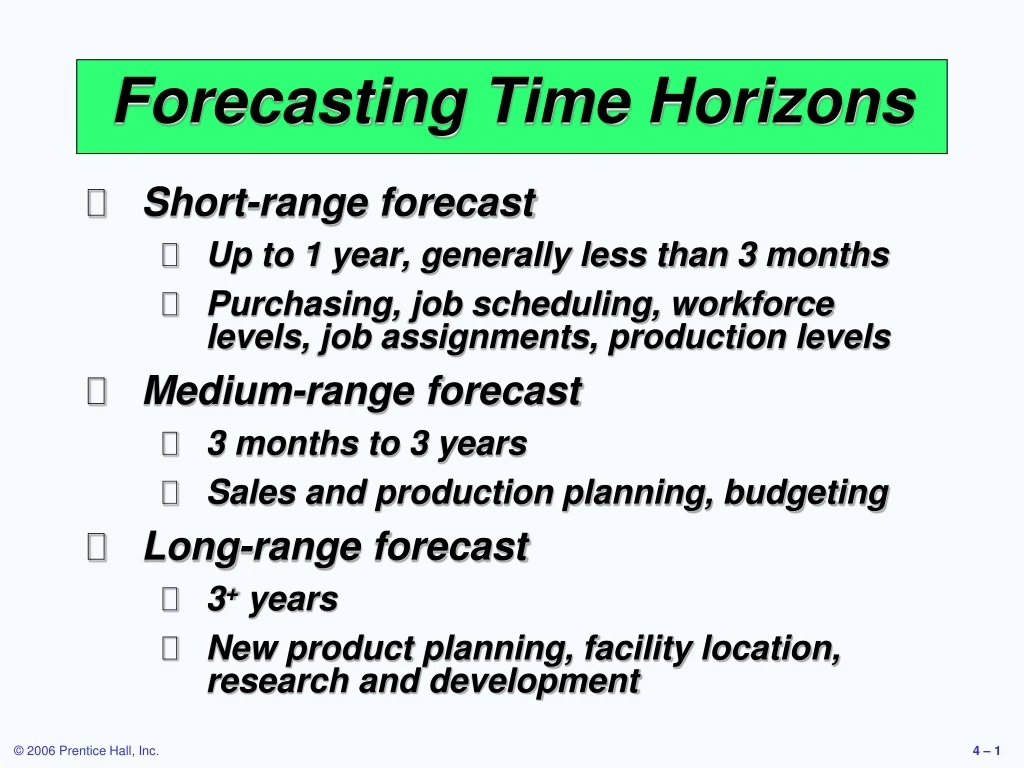
Forecasting Time Horizons • Short-range forecast • Up to 1 year, generally less than 3 months • Purchasing, job scheduling, workforce levels, job assignments, production levels • Medium-range forecast • 3 months to 3 years • Sales and production planning, budgeting • Long-range forecast • 3+ years • New product planning, facility location, research and development
Trend Cyclical Seasonal Random Time Series Components
Trend component Seasonal peaks Actual demand Demand for product or service Average demand over four years Random variation | | | | 1 2 3 4 Year Components of Demand Figure 4.1
Moving Average Forecast 30 – 28 – 26 – 24 – 22 – 20 – 18 – 16 – 14 – 12 – 10 – Actual Sales Shed Sales | | | | | | | | | | | | J F M A M J J A S O N D Graph of Moving Average
225 – 200 – 175 – 150 – Actual demand a = .5 Demand a = .1 | | | | | | | | | 1 2 3 4 5 6 7 8 9 Quarter Impact of Different
Actual observation (y value) Deviation7 Deviation5 Deviation6 Deviation3 Values of Dependent Variable Deviation4 Deviation1 Deviation2 ^ Trend line, y = a + bx Time period Least Squares Method Figure 4.4
Actual observation (y value) Deviation7 Deviation5 Deviation6 Deviation3 Values of Dependent Variable Deviation4 Deviation1 Deviation2 ^ Trend line, y = a + bx Time period Least Squares Method Least squares method minimizes the sum of the squared errors (deviations) Figure 4.4
Time Electrical Power Year Period (x) Demand x2 xy 1999 1 74 1 74 2000 2 79 4 158 2001 3 80 9 240 2002 4 90 16 360 2003 5 105 25 525 2004 6 142 36 852 2005 7 122 49 854 ∑x = 28 ∑y = 692 ∑x2 = 140 ∑xy = 3,063 x = 4 y = 98.86 3,063 - (7)(4)(98.86) 140 - (7)(42) a = y - bx = 98.86 - 10.54(4) = 56.70 ∑xy - nxy ∑x2 - nx2 b = = = 10.54 Least Squares Example
Time Electrical Power Year Period (x) Demand x2 xy 1999 1 74 1 74 2000 2 79 4 158 2001 3 80 9 240 2002 4 90 16 360 2003 5 105 25 525 2004 6 142 36 852 2005 7 122 49 854 Sx = 28 Sy = 692 Sx2 = 140 Sxy = 3,063 x = 4 y = 98.86 The trend line is ^ y = 56.70 + 10.54x 3,063 - (7)(4)(98.86) 140 - (7)(42) a = y - bx = 98.86 - 10.54(4) = 56.70 Sxy - nxy Sx2 - nx2 b = = = 10.54 Least Squares Example
Trend line, y = 56.70 + 10.54x 160 – 150 – 140 – 130 – 120 – 110 – 100 – 90 – 80 – 70 – 60 – 50 – ^ Power demand | | | | | | | | | 1999 2000 2001 2002 2003 2004 2005 2006 2007 Year Least Squares Example
^ y = a + bx ^ where y = computed value of the variable to be predicted (dependent variable) a = y-axis intercept b = slope of the regression line x = the independent variable though to predict the value of the dependent variable Associative Forecasting Forecasting an outcome based on predictor variables using the least squares technique
Sales Local Payroll ($000,000), y ($000,000,000), x 2.0 1 3.0 3 2.5 4 2.0 2 2.0 1 3.5 7 4.0 – 3.0 – 2.0 – 1.0 – Sales | | | | | | | 0 1 2 3 4 5 6 7 Area payroll Associative Forecasting Example
Sales, y Payroll, x x2 xy 2.0 1 1 2.0 3.0 3 9 9.0 2.5 4 16 10.0 2.0 2 4 4.0 2.0 1 1 2.0 3.5 7 49 24.5 ∑y = 15.0 ∑x = 18 ∑x2 = 80 ∑xy = 51.5 ∑xy - nxy ∑x2 - nx2 x = ∑x/6 = 18/6 = 3 b = = = .25 y = ∑y/6 = 15/6 = 2.5 a = y - bx = 2.5 - (.25)(3) = 1.75 51.5 - (6)(3)(2.5) 80 - (6)(32) Associative Forecasting Example
^ y = 1.75 + .25x 4.0 – 3.0 – 2.0 – 1.0 – 3.25 Sales | | | | | | | 0 1 2 3 4 5 6 7 Area payroll Associative Forecasting Example Sales = 1.75 + .25(payroll) If payroll next year is estimated to be $600 million, then: Sales = 1.75 + .25(6) Sales = $325,000
4.0 – 3.0 – 2.0 – 1.0 – 3.25 Sales | | | | | | | 0 1 2 3 4 5 6 7 Area payroll Standard Error of the Estimate • A forecast is just a point estimate of a future value • This point is actually the mean of a probability distribution Figure 4.9
∑(y - yc)2 n - 2 Sy,x = Standard Error of the Estimate where y = y-value of each data point yc = computed value of the dependent variable, from the regression equation n = number of data points
∑y2 - a∑y - b∑xy n - 2 Sy,x = Standard Error of the Estimate Computationally, this equation is considerably easier to use We use the standard error to set up prediction intervals around the point estimate
39.5 - 1.75(15) - .25(51.5) 6 - 2 ∑y2 - a∑y - b∑xy n - 2 Sy,x = = 4.0 – 3.0 – 2.0 – 1.0 – 3.25 Sales | | | | | | | 0 1 2 3 4 5 6 7 Area payroll Standard Error of the Estimate Sy,x = .306 The standard error of the estimate is $30,600 in sales
Correlation • How strong is the linear relationship between the variables? • Correlation does not necessarily imply causality! • Coefficient of correlation, r, measures degree of association • Values range from -1 to +1
nSxy - SxSy [nSx2 - (Sx)2][nSy2 - (Sy)2] r = Correlation Coefficient
y n∑xy - ∑x∑y [n∑x2 - (∑x)2][n∑y2 - (∑y)2] r = x (a) Perfect positive correlation: r = +1 (b) Positive correlation: 0 < r < 1 y y y x x (d) Perfect negative correlation: r = -1 (c) No correlation: r = 0 x Correlation Coefficient
Correlation • Coefficient of Determination, r2, measures the percent of change in y predicted by the change in x • Values range from 0 to 1 • Easy to interpret For the Nodel Construction example: r = .901 r2 = .81
^ y = a + b1x1 + b2x2 … Multiple Regression Analysis If more than one independent variable is to be used in the model, linear regression can be extended to multiple regression to accommodate several independent variables Computationally, this is quite complex and generally done on the computer
^ y = 1.80 + .30x1 - 5.0x2 Multiple Regression Analysis In the Nodel example, including interest rates in the model gives the new equation: An improved correlation coefficient of r = .96 means this model does a better job of predicting the change in construction sales Sales = 1.80 + .30(6) - 5.0(.12) = 3.00 Sales = $300,000
Monitoring and Controlling Forecasts • Measures how well the forecast is predicting actual values • Ratio of running sum of forecast errors (RSFE) to mean absolute deviation (MAD) • Good tracking signal has low values • If forecasts are continually high or low, the forecast has a bias error Tracking Signal
∑(actual demand in period i - forecast demand in period i) (∑|actual - forecast|/n) RSFE MAD Tracking signal = Tracking signal = Monitoring and Controlling Forecasts
Signal exceeding limit Tracking signal + 0 MADs – Upper control limit Acceptable range Lower control limit Time Tracking Signal
Cumulative Absolute Absolute Actual Forecast Forecast Forecast Qtr Demand Demand Error RSFE Error Error MAD 1 90 100 -10 -10 10 10 10.0 2 95 100 -5 -15 5 15 7.5 3 115 100 +15 0 15 30 10.0 4 100 110 -10 -10 10 40 10.0 5 125 110 +15 +5 15 55 11.0 6 140 110 +30 +35 30 85 14.2 Tracking Signal Example
TrackingSignal(RSFE/MAD) Cumulative Absolute Absolute Actual Forecast Forecast Forecast Qtr Demand Demand Error RSFE Error Error MAD -10/10 = -1 -15/7.5 = -2 0/10 = 0 -10/10 = -1 +5/11 = +0.5 +35/14.2 = +2.5 1 90 100 -10 -10 10 10 10.0 2 95 100 -5 -15 5 15 7.5 3 115 100 +15 0 15 30 10.0 4 100 110 -10 -10 10 40 10.0 5 125 110 +15 +5 15 55 11.0 6 140 110 +30 +35 30 85 14.2 Tracking Signal Example The variation of the tracking signal between -2.0 and +2.5 is within acceptable limits