Download
1 / 30
300 likes | 390 Vues
Learn about spatial analysis using raster data in GIS, including types of analysis, grid structure, and applications. Discover how to conduct spatial analysis and apply it to real-world problems with step-by-step guidance.

E N D
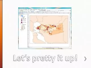
Border around project area Big circles… and semi-transparent Color distinction is clear Everything else is hardly noticeable… but it’s there
Introduction to GIS – Yoh Kawano Spatial Analysis
Spatial analysis refers to the formal techniques to conduct analysis using their topological, geometric, or geographic properties. • In a narrower sense, spatial analysis is the process of analyzing geographic data. • Types of spatial analysis you have already been doing: • Buffering • Select by location Spatial Analysis
Layers can be overlaid - placed one over the other based on a shared geographic reference – allows analysis of the relationships between layers
Why do we have to use raster data? • Vector data (points, lines and polygons) are limited to only certain spatial analyses • Point in polygon (which points are within • Line intersections • Vector data only knows about the space it occupies • Raster data covers the entire region • Provides a more powerful format for advanced spatial and statistical analysis Raster Data
A matrix of cells • Rows and columns (grid) • Examples: aerial photographs, digital photos, scanned maps • Examples in spatial analyst… Raster Data
As basemaps • As surface maps • As thematic maps Types of Raster Data
Grid size is defined by extent, spacing and no data value information • Number of rows, number of column • Cell sizes (X and Y) • Top, left , bottom and right coordinates • Grid values • Real (floating decimal point) • Integer (may have associated attribute table) The grid data structure
Cell size Number of rows NODATA cell (X,Y) Number of Columns Definition of a Grid
derive new information from your existing data, • analyze spatial relationships, • build spatial models, and • perform complex raster operations. So now that I know what a raster is… what can I do with it?
Find suitable locations • Model and visualize crime patterns • Analyze transportation corridors • Perform land use analysis • Conduct risk assessments • Predict fire risk • Determine erosion potential • Determine pollution levels • Perform crop yield analysis Applications of spatial analysis
Step 1: State the Problem • Find the most suitable location for a new long-term care facility in Long Beach • Step 2: Identify the Parameters and Weight • Supply: needs to be far from existing facilities (weighted by number of beds in the facilities) (25%) • Demand: number of persons over 65 (50%) • Access: close to major streets (25%) • Step 3: Prepare Your Input Datasets • Long Beach Facilities (point) • Census Tracts – Age>65 (polygon) • Major Streets (line) • Step 4: Perform the Analysis How to find “suitable” locations
ArcCatalog: • Make sure all your layers are in the same projection (eg: UTM Zone 11N) • ArcMap: • Load all your layers, double check that you are on the right projection and units (eg: miles) • Turn on Spatial Analyst Toolbar • Set the Environment (very important, ensures that raster layers have the same cell size!) • Load your indicator layers • “Rasterize” your layers (Ex: Kernel Density, Feature to Raster, Euclidean Distance) • Reclassify • Apply weights • Generate final raster ArcGIS Workflow
Step 1 Ensure that each layer in your project has the SAME projection
Step 2 Check the map units *Even if you change the “display” units, spatial analysis will be conducted using the “map” units
Right click Step 3 Access ArcToolbox Environments
Step 4 Set the environment Processing ExtentUsually set this to the extent of your project, or the largest layer Raster AnalysisCell size and Mask
Best site for new facility 25% 50% 25% Far from existing facilities Close to areas with high numbers of senior citizens Close to major streets Kernel Density on Number of Beds Feature to Raster on Age>65 Euclidean Distance Long Beach Facilities Long Beach Census Tracts Long Beach Major Roads
Spatial Analysis Tools > Density > Kernel Density Example: Kernel Density
Spatial Analysis Tools > Distance > Euclidean Distance Example: Euclidean Distance
Conversion Tools > To Raster > Feature to Raster Example: Feature to Raster
Kernel Density on Number of Beds 3 3 3 Reclassify: 3 most desirable 1 = least desirable 1 3 2 1 1 2 Long Beach Facilities Feature to Raster on Age>65 Reclassify: 3 most desirable 1 = least desirable 1 1 3 1 2 3 2 2 3 Long Beach Census Tracts 2 1 3 Euclidean Distance Reclassify: 3 most desirable 1 = least desirable 2 1 1 2 2 1 Long Beach Major Roads Spatial Analysis Tools > Reclass > Reclassify
3 3 3 25% .75 .75 .75 Long Beach Facilities 1 3 2 .25 .75 .5 1 1 2 .25 .25 .5 1 1 3 .5 .5 1.5 50% Long Beach Census Tracts 1 2 3 .5 1 1.5 2 2 3 1 1 1.5 2 1 3 .5 .25 .75 25% Long Beach Major Roads 2 1 1 .5 .25 .25 2 2 1 .5 .5 .25 1.75 1.5 3 1.25 2 2.25 Spatial Analysis Tools > Map Algebra > Raster Calculator 1.75 1.75 2.25