Chapter 6 Control Charts for Attributes
Chapter 6 Control Charts for Attributes. Introduction. It is not always possible or practical to use measurement data Number of non-conforming parts for a given time period Clerical operations The objective is to continually reduce the number of non-conforming units.

Chapter 6 Control Charts for Attributes
E N D
Presentation Transcript
Introduction • It is not always possible or practical to use measurement data • Number of non-conforming parts for a given time period • Clerical operations • The objective is to continually reduce the number of non-conforming units. • Control charts for attributes might be used in conjunction with measurement charts. They should be used alone only when there is no other choice.
Terminology • Fraction of non-conforming units (ANSI standard) • Fraction or percentage of… • non-conforming, or defective, or rejected • Non-conformity • Defect
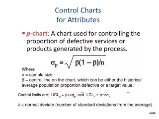
6.1 Charts for Non-conforming Units • Charts based on fraction of non-conforming units: p-chart • Charts based on number of non-conforming units: np-chart • Assumptions using control limits at : • Normal approximation to the binomial distribution is adequate • non-conformities occur independently • Extrabinomial variation (overdispersion) can occur when the independency assumption was violated
6.1 Charts for Non-conforming Units • Let X be the number of non-conforming unit in a sample of size n, and denote the proportion of such units, and Will be approximately distributed as N(=0, =1) when n is at least moderately large and p does not differ greatly from 0.5. (6.1) (6.2)
6.1.1 np-Chart • Control limits for np-chart are • Rule-of-thumb: np>5; n(1-p)>5 • Example: for n=400, p=.10; UCL=58, LCL=22 • Binomial: P(X>58)=0.0017146; P(X<22)=0.0004383 • The adequacy of the approximation depends primarily on p. • If p=.09, P(X<22)=0.00352185, ARL=284 • If p=.08, P(X<22)=0.02166257, ARL=46 • LCL is not very sensitive to quality improvement • UCL has meaning only for defensive purpose • LCL will be 0 if p<9/(9+n); or n<9(1-p)/p (6.3)
6.1.2 p-Chart • Control limits for np-chart are • A scaled version of np-chart (6.4)
6.1.3 Stage 1 and Stage 2 Use of p-Charts and np-Charts • Need to estimate p in order to determine the sample size • If p~.01, n should be 900 or larger to ensure LCL • An estimate of p would be obtained as • 3-sigma limits for np-chart • UCL=20.315, LCL=.885
Table 6.1 No. of Non-conforming Transistors out of 1000 Inspected
6.1.4 Alternative Approaches • Alternatives to the use of 3-sigma limits: (since the LCL generally too small) • Arcsin Transformation • Q-Chart • Regression-based Limits • ARL-Unbiased Charts
6.1.4.1 ArcsinTransformation Will be approximately normal with mean and variance For each sample of size n, one would plot the value of y on a control chart with the midline at and the control limits: (6.5) (6.6)
6.1.4.1 ArcsinTransformation: Example When n=400 and p=.10, the control limits would be: UCL=.39675 (X=59.29), LCL=.24675 (X=23.53) Bino(X60)=0.001052825; Bino(X23)=0.00167994 3-sigma limits: UCL=58, LCL=22 Bino(X59)=0.001714566; Bino(X21)=0.000438333 Table 6.2, Table 6.3 Comparison of np-chart based on 3-sigma and arcsin transformation Table 6.4 Minimum sample size necessary for LCL to exist
6.1.4.2 Q-Chart • Let denote • If 3-sigma limits are used, the statistics are plotted against control limits of 3, where denotes the normal cumulative distribution function (cdf) and p is known. • Q-charts have LTA less than .00135, and UTA greater than .00135. • Arcsin approach gives a better approximation to the LTA.
6.1.4.3 Regression-based Limits • Regression-based Limits for an np-chart • The objective is to minimize • Will produce the optimal limits when p~.01 (6.7)
6.1.4.4 ARL-Unbiased Charts • Control limits are such that the in-control ARL is larger than any of the parameter-change ARLs • Problem with skewed distributions
6.1.5 Using Software to Obtain Probability Limits for p- and np-Charts • INVCDF probibility; (In Minitab) • Possible distributions and their parameters are • bernoulli p = k • binomial n = k p = k • poissonmu=k • normal [mu=k [sigma=k]] • uniform [a=k b=k] • t df=k • f df1=k df2=k • chisquaredf=k
6.1.6 Variable Sample Size • The variable limits for the p-chart • Standardized p-chart, with UCL=3, LCL=-3 (6.8)
6.1.7 Charts Based on the Geometric and Negative Binomial Distributions • The use of p-chart when p is extremely small is inadvisable • It is preferable to plot the number of plotted points until k non-conforming units are observed. • If k=1, it is geometric distribution • However, these limits are not ARL-unbiased.
6.1.8 Overdispersion • The actual variance of X (or ) is greater than the variance obtained using the binomial distribution. • Causes of overdispersion: • Non-constant p: • Autocorrelation
6.2 Charts for Non-conformities • A unit of production can have one or more non-conformities without being labeled a non-conforming unit. • non-conformities can occur in non-manufacturing applications
6.2.1 c-Chart • C-chart can be used to control the number of non-conformities per sample of inspection units. • Control limits for c-chart are • Poisson distribution • Adequacy of normal approximation to Poisson • should be at least 5 • No LCL when (6.9)
6.2.4 Regression-based Limits • Regression-based Limits for a c-chart • For • LCL exists when • For the previous example, , LCL=1.66, UCL=16.42 • Regression-based limits are superior to the transformation limits (6.10)
6.2.5 Using Software to Obtain Probability Limits for c-Charts • INVCDF probibility; (In Minitab) • Possible distributions and their parameters are • bernoulli p = k • binomial n = k p = k • poissonmu=k • normal [mu=k [sigma=k]] • uniform [a=k b=k] • t df=k • f df1=k df2=k • chisquaredf=k
6.2.6 u-Chart • Used when the area of opportunity for the occurrence of non-conformities does not remain constant. • The control limits for the u-chart, • Use instead of n with variable sample size • Alternatively, use if individual sample size differs from the average no more than 25% (6.11)
6.2.6 u-Chart with Transformation • For constant sample size, • For variable sample size,
6.2.6.1 Regression-based Limitsfor u-chart • Let the UCL for a c-chart be represented by and LCL be represented by • Solve for and • For variable the control limits for the u-chart would be
6.2.6.1 Regression-based Limitsfor u-chart Example • Let ; • Let ; • The control limits for the u-chart would be
6.2.7 Overdispersion • If overdispersion is found to exist, the negative binomial distribution may be a suitable model.
6.2.8 D-Chart • C-chart can be used to chart a single type of non-conformity, or to chart the sum of different types of non-conformities with equal weight • If different weights (demerits) can be assigned, use D-charts • Assuming 3 different types of non-conformities (c1, c2, c3) with weights (w1, w2, w3), then D represents the number of demerits • Assuming 1, D will not have a Poisson distribution
6.2.8 D-Chart • For different types of independent non-conformities Where is the mean of , and estimated by • Let represent the number of non-conformities of type in inspection unit , then • The 3-sigma control limits for D-chart are
6.2.8 Du-Chart for Variable Units • If each sample contains more than 1 inspection unit and it is desired to chart the number of demerits per inspection unit, then the counterpart of u-chart would be produced. • is the number of non-conformities of type per inspection unit in a sample that contains such units • If samples are available
6.2.8 Du-Chart for Variable Units • For different types of independent non-conformities Where is the mean of , and estimated by • The 3-sigma control limits for D-chart are