Download
1 / 66
1.77k likes | 4.12k Vues
Control Charts for Variables. EBB 341 Quality Control. Variation. There is no two natural items in any category are the same. Variation may be quite large or very small. If variation very small, it may appear that items are identical, but precision instruments will show differences.

E N D
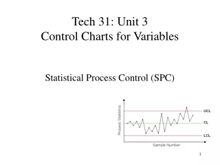
Control Charts for Variables EBB 341 Quality Control
Variation • There is no two natural items in any category are the same. • Variation may be quite large or very small. • If variation very small, it may appear that items are identical, but precision instruments will show differences.
3 Categories of variation • Within-piece variation • One portion of surface is rougher than another portion. • Apiece-to-piece variation • Variation among pieces produced at the same time. • Time-to-time variation • Service given early would be different from that given later in the day.
Source of variation • Equipment • Tool wear, machine vibration, … • Material • Raw material quality • Environment • Temperature, pressure, humadity • Operator • Operator performs- physical & emotional
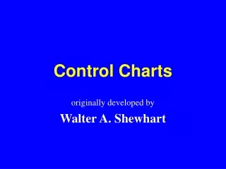
Control Chart Viewpoint • Variation due to • Common or chance causes • Assignable causes • Control chart may be used to discover “assignable causes”
Some Terms • Run chart - without any upper/lower limits • Specification/tolerance limits - not statistical • Control limits - statistical
Control chart functions • Control charts are powerful aids to understanding the performance of a process over time. Output PROCESS Input What’s causing variability?
Control charts identify variation • Chance causes - “common cause” • inherent to the process or random and not controllable • if only common cause present, the process is considered stable or “in control” • Assignable causes - “special cause” • variation due to outside influences • if present, the process is “out of control”
Control charts help us learn more about processes • Separate common and special causes of variation • Determine whether a process is in a state of statistical control or out-of-control • Estimate the process parameters (mean, variation) and assess the performance of a process or its capability
Control charts to monitor processes • To monitor output, we use a control chart • we check things like the mean, range, standard deviation • To monitor a process, we typically use two control charts • mean (or some other central tendency measure) • variation (typically using range or standard deviation)
Types of Data • Variable data • Product characteristic that can be measured • Length, size, weight, height, time, velocity • Attribute data • Product characteristic evaluated with a discrete choice • Good/bad, yes/no
Control chart for variables • Variables are the measurablecharacteristics of a product or service. • Measurement data is taken and arrayed on charts.
Control charts for variables • X-bar chart • In this chart the sample means are plotted in order to control the mean value of a variable (e.g., size of piston rings, strength of materials, etc.). • R chart • In this chart, the sample ranges are plotted in order to control the variability of a variable. • S chart • In this chart, the sample standard deviations are plotted in order to control the variability of a variable. • S2 chart • In this chart, the sample variances are plotted in order to control the variability of a variable.
X-bar and R charts • The X- bar chart is developed from the average of each subgroup data. • used to detect changes in the mean between subgroups. • The R- chart is developed from the ranges of each subgroup data • used to detect changes in variation within subgroups
Control chart components • Centerline • shows where the process average is centered or the central tendency of the data • Upper control limit (UCL) and Lower control limit (LCL) • describes the process spread
The Control Chart Method X bar Control Chart: UCL = XDmean + A2 x Rmean LCL = XDmean - A2 x Rmean CL = XDmean R Control Chart: UCL = D4 x Rmean LCL = D3 x Rmean CL = Rmean Capability Study: PCR = (USL - LSL)/(6s); where s = Rmean /d2
Control Chart Examples UCL Nominal Variations LCL Sample number
Define the problem • Use other quality tools to help determine the general problem that’s occurring and the process that’s suspected of causing it. Select a quality characteristic to be measured • Identify a characteristic to study - for example, part length or any other variable affecting performance.
Choose a subgroup size to be sampled • Choose homogeneous subgroups • Homogeneous subgroups are produced under the same conditions, by the same machine, the same operator, the same mold, at approximately the same time. • Try to maximize chance to detect differences between subgroups, while minimizing chance for difference with a group.
Collect the data • Generally, collect 20-25 subgroups (100 total samples) before calculating the control limits. • Each time a subgroup of sample size n is taken, an average is calculated for the subgroup and plotted on the control chart.
Determine trial centerline • The centerline should be the population mean, • Since it is unknown, we use X Double bar, or the grand average of the subgroup averages.
Determine trial control limits - Xbar chart • The normal curve displays the distribution of the sample averages. • A control chart is a time-dependent pictorial representation of a normal curve. • Processes that are considered under control will have 99.73% of their graphed averages fall within 6.
Determine trial control limits - R chart • The range chart shows the spread or dispersion of the individual samples within the subgroup. • If the product shows a wide spread, then the individuals within the subgroup are not similar to each other. • Equal averages can be deceiving. • Calculated similar to x-bar charts; • Use D3and D4 (appendix 2)
Example: Control Charts for Variable Data Slip Ring Diameter (cm) Sample 1 2 3 4 5 X R 1 5.02 5.01 4.94 4.99 4.96 4.98 0.08 2 5.01 5.03 5.07 4.95 4.96 5.00 0.12 3 4.99 5.00 4.93 4.92 4.99 4.97 0.08 4 5.03 4.91 5.01 4.98 4.89 4.96 0.14 5 4.95 4.92 5.03 5.05 5.01 4.99 0.13 6 4.97 5.06 5.06 4.96 5.03 5.01 0.10 7 5.05 5.01 5.10 4.96 4.99 5.02 0.14 8 5.09 5.10 5.00 4.99 5.08 5.05 0.11 9 5.14 5.10 4.99 5.08 5.09 5.08 0.15 10 5.01 4.98 5.08 5.07 4.99 5.03 0.10 50.09 1.15
Calculation From Table above: • Sigma X-bar = 50.09 • Sigma R = 1.15 • m = 10 Thus; • X-Double bar = 50.09/10 = 5.009 cm • R-bar = 1.15/10 = 0.115 cm Note: The control limits are only preliminary with 10 samples. It is desirable to have at least 25 samples.
Trial control limit • UCLx-bar = X-D bar + A2 R-bar = 5.009 + (0.577)(0.115) = 5.075 cm • LCLx-bar = X-D bar - A2 R-bar = 5.009 - (0.577)(0.115) = 4.943 cm • UCLR = D4R-bar = (2.114)(0.115) = 0.243 cm • LCLR = D3R-bar = (0)(0.115) = 0 cm For A2, D3, D4: see Table B, Appendix n = 5
3-Sigma Control Chart Factors Sample size X-chart R-chart nA2D3D4 2 1.88 0 3.27 3 1.02 0 2.57 4 0.73 0 2.28 5 0.58 0 2.11 6 0.48 0 2.00 7 0.42 0.08 1.92 8 0.37 0.14 1.86
Calculation From Table 5.2: • Sigma X-bar = 160.25 • Sigma R = 2.19 • m = 25 Thus; • X-double bar = 160.25/29 = 6.41 mm • R-bar = 2.19/25 = 0.0876 mm
Trial control limit • UCLx-bar = X-double bar + A2R-bar = 6.41 + (0.729)(0.0876) = 6.47 mm • LCLx-bar = X-double bar - A2R-bar = 6.41 – (0.729)(0.0876) = 6.35 mm • UCLR = D4R-bar = (2.282)(0.0876) = 0.20 mm • LCLR = D3R-bar = (0)(0.0876) = 0 mm For A2, D3, D4: see Table B Appendix, n = 4.
Revised CL & Control Limits Calculation based on discarding subgroup 4 & 20 (X-bar chart) and subgroup 18 for R chart: = (160.25 - 6.65 - 6.51)/(25-2) = 6.40 mm = (2.19 - 0.30)/25 - 1 = 0.079 = 0.08 mm
New Control Limits New value: • Using standard value, CL & 3 control limit obtained using formula:
From Table B: • A = 1.500 for a subgroup size of 4, • d2 = 2.059, D1 = 0, and D2 = 4.698 Calculation results:
Trial Control Limits & Revised Control Limit Revised control limits UCL = 6.46 CL = 6.40 LCL = 6.34 UCL = 0.18 CL = 0.08 LCL = 0
Revise the charts • In certain cases, control limits are revised because: • out-of-control points were included in the calculation of the control limits. • the process is in-control but the within subgroup variation significantly improves.
Revising the charts • Interpret the original charts • Isolate the causes • Take corrective action • Revise the chart • Only remove points for which you can determine an assignable cause
Process in Control • When a process is in control, there occurs a natural pattern of variation. • Natural pattern has: • About 34% of the plotted point in an imaginary band between 1s on both side CL. • About 13.5% in an imaginary band between 1s and 2s on both side CL. • About 2.5% of the plotted point in an imaginary band between 2s and 3s on both side CL.
LSL USL Mean -3 -2 -1 +1 +2 +3 68.26% 95.44% 99.74% -3 +3 CL The Normal Distribution = Standard deviation
34.13% of data lie between and 1 above the mean (). • 34.13% between and 1 below the mean. • Approximately two-thirds (68.28 %) within 1 of the mean. • 13.59% of the data lie between one and two standard deviations • Finally, almost all of the data (99.74%) are within 3of the mean.
Normal Distribution Review • Define the 3-sigma limits for sample means as follows: • What is the probability that the sample means will lie outside 3-sigma limits? • Note that the 3-sigma limits for sample means are different from natural tolerances which are at