Robust adaptive variable structure control
Robust adaptive variable structure control. Yoni Habuba Amichay Israel. adviser : Mark Moulin. introduction.

Robust adaptive variable structure control
E N D
Presentation Transcript
Robust adaptive variable structure control Yoni Habuba Amichay Israel adviser : Mark Moulin
introduction Future spacecraft will be expected to achieve highly accurate pointing, fast slewing, and other fast maneuvers from large initial conditions and in the presence of large environmental disturbances, measurement noise, large uncertainties, subsystem , component failures and control input saturation.
Introduction (Cont.) In this project we propose globally stable control algorithms for robust stabilization of spacecraft in the presence of controls input saturation, parametric uncertainty, and external disturbances.
Introduction (Cont.) We will compare between 6 control algorithms. One of the controllers is a simple proportional, the other - 5 of the 6 control algorithms are based on variable structure control design and have the following properties: fast and accurate response in the presence of bounded external disturbances and parametric uncertainty explicit accounting for control input saturation Computational simplicity and straightforward tuning.
Equation set J denotes inertia matrix U denotes the control torques Ω denotes the inertial angular velocity ε and ε0 denote the Euler parameters The purpose is to stabilize Ω ,ε and ε0
Sliding surface • In the context of spacecraft control, the control-based sliding mode control design is based on the use of the following sliding surface: where k > 0 is a scalar
Controller's presentation • Equivalent control-based sliding mode controller • Sliding mode control under control input saturation using an approximate sign function • Sliding mode control under control input saturation using an accurate sign function • Combination between the sliding surface and proportional controller • proportional • Adaptive variable structure controller
Controller 1 • Equivalent control-based sliding mode controller • u = ueq + uvs • Where ueq denotes the equivalent control component and is chosen to ensure that s(t) = 0 for all time . return
Comparison between Controller 2 and Controller 3Sliding mode control under control input saturation using an approximate sign function Controller 3 Controller 2 NOTE: controller 3 has a chattering problem therefore we will use controller 2 only from now on return
Controller 4 • Combination between the sliding surface and proportional controller • u=ueq +upr • Where ueq denotes the equivalent control component and is chosen to ensure that s(t) = 0 for all time . return
Controller 5 • proportional • Controller law is • For getting the gain vector we made linearization of the system around the point: • After the linearization we determined the poles we used Ackerman's method for getting the gain vector. return
Controller 6 • Adaptive variable structure controller • Controller 6 is the similar to Controller 2 i.e. • but the different is that k in the equation • is time depend i.e. • while γ >0 denote the adaptive gain . return
Simulation • The initial condition for all controllers: • W(0)=[29 29 29] • e(0) =[0.4 0.2 0.4 ] • eo(0)=0.8 • The inertia matrix is
Disturbances rejection • We have checked the response of the difference controllers to a certain disturbances: • Square wave, 30pp, f=0.5 Hz. • Sinus wave, 30pp, f=0.5 Hz. • Triangle wave, 30pp, f=0.5 Hz. • We will present the sinus disturbance.
W1 - sin source Yellow - Controller1 Magenta –Controller2 Cyan – Controller4 Red – Controller5 Blue – Controller6
e1 - sin source Yellow - Controller1 Magenta –Controller2 Cyan – Controller4 Red – Controller5 Blue – Controller6
U1 - sin source Yellow - Controller1 Magenta –Controller2 Cyan – Controller4 Red – Controller5 Blue – Controller6
Controller’s effectiveness to different parameters We have cheeked the parameters in the presence of the following disturbances: • Square wave 20pp, 40pp, 60pp, f=0.5 Hz • Inside disturbance 2pp f=0.5 Hz . We will present the parameters for disturbance 1 . • We have checked the following parameters: • Max value • -steady error state. • Tsettle • Umax • Robustness to changing the initial conditions.
Conclusions • larger disturbance causes larger εss • The controllers 2, 6 which have only a non linear controller do not converge while the disturbance amplitude is 60 because it is ~Umax=70. • another conclusion that can’t be seen from the table and graphs but we have checked it by simulation The controllers are more effective for larger frequencies (~ 100 Hz)
Robust to changing the initial conditions • We have noticed that the controllers have a problem to settle the system while the initial conditions are too large • We have checked the for the different controllers
Discussion about the internal parameters of controllers 2,6 • We have discussed the following parameters regarded to controllers 2 and 6 : • Discussion about limitation of k in controller 2 • Discussion about γ and k(0) in controller 6 We will present the discussion about γ in controller 6
Ω1 ε1 K(t)
Ω1 ε1 K(t)
Conclusion It can be seen immediately that for γ =0.01 • e(t) - don’t converge to zero. • k(t) - converge to zero
Explanation This controller only guarantees that k(t)Xe(t) ,but not necessarily e(t) ,will converge to zero. If k(t) converge to zero faster than e(t) ,then e(t) may converge to some nonzero constant value. To ensure that e(t) will converge to zero, one need to keep k(t) from converging to zero. This can be achieved by using a sufficiently small γ such that k(t) changes slowly and that and hence will not deviate too much from its initial value.