Download
1 / 37
370 likes | 508 Vues
Application of Quasi-Newton Algorithms in Optimal Design . Sebastian Ueckert, Joakim Nyberg, Andrew C. Hooker. Pharmacometrics Research Group Department of Pharmaceutical Biosciences Uppsala University Sweden. Outline. Optimizing Designs Introduction: Quasi-Newton Methods (QNMs)

E N D
Application of Quasi-Newton Algorithms in Optimal Design Sebastian Ueckert, Joakim Nyberg, Andrew C. Hooker Pharmacometrics Research Group Department of Pharmaceutical Biosciences Uppsala University Sweden
Outline • Optimizing Designs • Introduction: Quasi-Newton Methods (QNMs) • Performance QNMs • Advantages QNMs • Laplace Approximation for Global Optimal Design • Using QNMs in Laplace Approximation
Optimizing a Design Model Parameters α Design variables x Data Estimation e.g. D-Optimal Design
Optimization • Interval methods True global optimizers Hard to implement Still under development • Stochastic methods • Simulated Annealing (SA), Ant colony optimization, Genetic Algorithm(GA) Easy to implement (SA) Marketing effective (GA) Slow No information about solution Heuristic
Optimization • Derivative free methods • Downhill Simplex Method No derivatives necessary Robust Slow Local
Gradient Based Methods Mathematically well understood Fast (if OFV calc not too expensive) Only local Complicated to implement • Steepest Descent • Conjugate Gradient
Newton Method Goal: Algorithm: Set xk=x0 Determine search direction Do line search along p* to find minimal xk+1 Set xk=xk+1 and go to 2
Newton Method Goal: Algorithm: Set xk=x0 Determine search direction Do line search along p* to find minimal xk+1 Set xk=xk+1 and go to 2 Calculate Hessian
Quasi-Newton Methods Problem: Calculation of Hessian is computationally expensive Approach: Use approx. Hessian and build up during search Algorithm: Set xk=x0, Bk=I Determine search direction Do line search along p* to find minimal xk+1 Set xk=xk+1, Bk=Bk+Uk and go to 2
Quasi-Newton Methods • Different methods for different updating formulas • Davidon–Fletcher–Powell (DFP) • Broyden-Fletcher-Goldfarb-Shanno (BFGS)
Constraints • Experiments usually come with practicality constraints e.g.: • Administered dose has to be smaller than X mg • Sampling times can only be taken until 8 h after dosing Box Constraints BFGS-B
BFGS-B Algorithm: Set xk=x0, Bk=I Determine search direction Project search direction vector on feasible region Do line search along p* to find minimal xk+1 respecting bounds Set xk=xk+1, Bk=Bk+Uk and go to 2
Comparison • Test Scenario • Model: • PKPD (1 cmp oral absorption; IMAX drug effect) • All parameters (ka,CL,V,IC50, E0, IMAX) with log-normal IIV 30% CV • PK parameters fixed • Combined error • Design: • 3 groups (40,30,30 subjects) • 1 PK and 1 PD sample per subject • Approach: • Generate random initial values • Optimize with steepest descent and BFGS
Results Runtime [s] Frequency[%] OFV
Design Sensitivity • Approximate Hessian matrix can be used to assess sensitivity of design (at no additional computational costs) • Diagonal of the inverse of the Hessian • Use approximate efficiency
Design Sensitivity - Visual Group 2 PD Group 1 PK Group 1 PD
Design Sensitivity - Numerical Group 1 PK Group 3 PK Group 2 PD
Global Optimal Design • Integral has to be evaluated • FIM occurs in integrand • For example ED optimal design: • Usually evaluated with Monte-Carlo integration Computationally intensive or imprecise
Laplace Approximation Algorithm: Minimize Calculate the Hessian Evaluate
Laplace-BFGS Approximation Algorithm: Minimize using BFGS algorithm Evaluate
Laplace-BFGS – Random Effects Problem: For variance parameter α ≥ 0 Approach: Perform optimization on log-domain Algorithm: Minimize using BFGS algorithm Rescale approximate Hessian Evaluate
Comparison • Comparison of 4 algorithms: • Monte Carlo integration with random sampling (MC-RS) • Monte Carlo integration with Latin hypercube sampling (MC-LHS) • Laplace integral approximation (LAPLACE) • Laplace integral approximation with BFGS Hessian (LAPLACE-BFGS) • Testing MC methods with 50 and 500 random samples
Comparison • Test Scenario • Model: • 1 cmp IV bolus • CL,V with log-normal IIV • Additive error • Design: • 20 subjects • 2 samples per subject • Parameter distribution: • Log-normal an all parameters (Fixed effect Var=0.05; Random Effect Var=0.09)
Results - OFV Mean OFV and non-parametric confidence intervals for different integration methods from 100 evaluations
Results - Design MC-RS 50 MC-LHS 50 LAPLACE MC-RS 500 MC-LHS 500 LAPLACE-BFGS
Results – Runtimes Runtime [s]
Conclusions • Quasi-Newton methods constitute fast alternative for continuous design variable optimization • Information about design sensitivity can be obtained with no additional cost • Global Optimal Design: • Monte-Carlo methods are easy and flexible but need high number of samples to give stable results • Laplace approximation constitutes fast alternative for priors with continuous probability distribution function • Laplace integral approximation with BFGS Hessian gave same sampling times with approx. 30% shorter runtimes
References • C.G. Broyden, “The Convergence of a Class of Double-rank Minimization Algorithms 1. General Considerations,” IMA J Appl Math, vol. 6, Mar. 1970, pp. 76-90. • R. Fletcher, “A new approach to variable metric algorithms,” The Computer Journal, vol. 13, 1970, p. 317. • D. Goldfarb, “A family of variable-metric methods derived by variational means,” Mathematics of Computation, 1970, pp. 23–26. • D.F. Shanno, “Conditioning of quasi-Newton methods for function minimization,” Mathematics of Computation, 1970, pp. 647–656. • R.H. Byrd, P. Lu, J. Nocedal, and C. Zhu, “A limited memory algorithm for bound constrained optimization,” SIAM J. Sci. Comput., vol. 16, 1995, pp. 1190-1208. • M. Dodds, A. Hooker, and P. Vicini, “Robust Population Pharmacokinetic Experiment Design,” Journal of Pharmacokinetics and Pharmacodynamics, vol. 32, Feb. 2005, pp. 33-64.