Optimal Design of Dynamic Experiments
950 likes | 1.17k Vues
“ The Systems Biology Modelling Cycle (supported by BioPreDyn) ” EMBL-EBI (Cambridge, UK), 12-15 May 2014. Optimal Design of Dynamic Experiments. Julio R. Banga IIM-CSIC, Vigo, Spain julio@iim.csic.es. Optimal Experimental Design (OED). Introduction OED: Why , what and how ?

Optimal Design of Dynamic Experiments
E N D
Presentation Transcript
“The Systems Biology Modelling Cycle (supported by BioPreDyn)” EMBL-EBI (Cambridge, UK), 12-15 May 2014 Optimal Design of Dynamic Experiments Julio R. Banga IIM-CSIC, Vigo, Spain julio@iim.csic.es
Optimal Experimental Design (OED) • Introduction • OED: Why, what and how? • Modelbuildingcycle • OED toimprovemodelcalibration • Formulation and examples • OED software and references
Modelling – considerations • Modelsstartswithquestions (purpose) and level of detail • Weneed a priori data & knowledgetobuild a 1st model • Wethenplan and perform new experiments, obtainnew data and refine themodel • Werepeatuntilstoppingcriterionsatisfied
Modelling – considerations • Weplan and perform new experiments, obtainnew data and refine themodel • But, how do we plan theseexperiments? • Optimal experimental design (OED) • Model-based OED
OED – Why? • Wewanttobuild a model • Wewantto use themodelforspecificpurposes (“modelsstartswithquestions”) • OED allowustoplan experimentsthatwill produce data withrichinformationcontent
OED - What ? • Weneedtotakeintoaccount: • (i) thepurpose of themodel, • (ii) the experimental degrees of freedom and constraints, • (iii) theobjective of the OED: • Parameterestimation • Modeldiscrimination • Modelreduction • …
OED – simple example • Wewanttobuild a 3D model of anobjectfrom 2D pictures
OED – simple example • Wewanttobuild a 3D model of anobjectfrom 2D pictures
OED – simple example • Wewanttobuild a 3D model of anobjectfrom 2D pictures • (i) purpose of themodel: a rough 3D representation of theobject, • (ii) experimental constraints: we can onlytake 2D snapshots • (iii) degrees of freedom: picturesfromanyangle • “Experiment” withminimumnumber of pictures?
OED – basicconsiderations • Thereis a minimumamount of information in the data neededtobuild a model • Thisdependson: • howdetailedwewantthemodeltobe • howcomplexthe original object (system) is • safeassumptionswe can make(e.g.symmetry in 3D object -> lesspicturesneeded)
Staticmodel Dynamicmodel
OED fordynamicmodels • Weneedtime-series datawithenoughinformationtobuild a model • Data fromdifferentcontexts, withenough time resolution
Dynamic process models Main characteristics: • Non-linear, dynamic models(i.e. batch or semi-batch processes) • Nonlinear constraints(safety and/or quality demands) • Distributed systems(T, c, etc.) • Coupled transport phenomena • Thus,mathematical models consist of sets of ODEs, DAEs, PDAEs, or even IPDAEs, with possible logic conditions (transitions, i.e. hybrid systems) • PDAEs models are usually transformed into DAEs (I.e. discretization methods, like FEM, NMOL, etc.)
Model building Data Experiment Solver Fitted Model Model
Modelbuilding Optimal Experimental Design Identifiability Analysis Parameter Estimation Data Experiment Solver Identifiability Analysis Fitted Model Model
Modelbuildingcycle Prior information OED Parameterestimation New experiments Modelselection and discrimination New data
Experimental design • Experimental degrees of freedom and constraints • Initialconditions • Dynamicstimuli: type and number of perturbations • Measurements • What? • When? (sampling times, experimentduration) • Howmanyreplicates? • Howmanyexperiments? • Etc.
Examples • Bacterialgrowth in batchculture • 3-step pathway • Oregonator
Example: Bacterialgrowth in batchculture Concentration of microorganisms Concentration of growth limiting substrate
Example: Bacterialgrowth in batchculture Maximum growth rate Decay rate coefficient Concentration of microorganisms Michaelis-Menten constant Concentration of growth limiting substrate Yield coefficient
Example: Bacterialgrowth in batchculture Experimental design: Initial conditions? What to measure? (concentration of microorganisms and substrate?) When to measure? (sampling times, experiment duration) How many experiments? How many replicates? Etc.
Example: Bacterialgrowth in batchculture Case A: 1 experiment 11 equidistant sampling times Duration: 10 hours Measurements of S and B
Example: Bacterialgrowth in batchculture Parameter estimation using GO method (eSS)
Example: Bacterialgrowth in batchculture Case B: 1 experiment 11 equidistant sampling times Duration: 10 hours Measurements of S only
Example: Bacterialgrowth in batchculture Good fit for substrate! But bad predictions for bacteria…
Example: Bacterialgrowth in batchculture Measuring both B and S…
Example: Bacterialgrowth in batchculture Measuring only S…
Example: Bacterialgrowth in batchculture So, for this case of 1 experiment, we should measure both B and S But confidence intervals are rather large… What happens if we consider a second experiment? (same experiment, but with different initial condition for S) mmax : 4.0940e-001 9.4155e-002 (23%); Ks : 6.6525e+000 3.3475e+000 (50%); Kd : 3.9513e-002 7.0150e-002 (177%); Y : 4.8276e-001 1.6667e-001 (34%);
Example: Bacterialgrowth in batchculture 1stexperiment 2ndexperiment mmax : 3.9542e-001 3.4730e-002 (9%) Ks : 5.3551e+000 9.1440e-001 (17%) Kd : 4.1657e-002 2.5753e-002 (62%) Y : 4.8529e-001 6.1227e-002 (13%); Great improvement with a second experiment ! BUT, can we do even better?
Example: Bacterialgrowth in batchculture 1stexperiment 2ndexperiment mmax : 3.9542e-001 3.4730e-002 (9%) Ks : 5.3551e+000 9.1440e-001 (17%) Kd : 4.1657e-002 2.5753e-002 (62%) Y : 4.8529e-001 6.1227e-002 (13%); Great improvement with a second experiment ! BUT, can we do even better? OPTIMAL EXPERIMENTAL DESIGN
Example: simple biochemicalpathway C.G. Moles, P. Mendes y J.R. Banga, 2003. Parameterestimation in biochemicalpathways: a comparison of global optimizationmethods. GenomeResearch., 13:2467-2474.
Example: simple biochemicalpathway • Parameter estimation: • 36 parameters • measurements: concentrations of 8 species • 16 experiments (different values of S y P)
Example: simple biochemicalpathway Experiments (S, P values) Initial conditions for all the experiments 21 measurements per experiment , tf = 120 s
Example: simple biochemicalpathway Multi-start local methods fail… Multi-start SQP
Example: simple biochemicalpathway Parameterestimation: again (some) global methods can failtoo…
2.5 0.5 0.4 2 0.3 1.5 Concentración M2 Concentración E1 0.2 1 0.1 0.5 0 0 20 40 60 80 100 120 0 0 20 40 60 80 100 120 tiempo tiempo Example: simple biochemicalpathway Parameterestimation: bestfit looks prettygoodbut…
Contours [p1, p6] Contours [p1, p4] Example: simple biochemicalpathway Identifiabilityproblems…
Practical identifiability problems are often due to data with poor information content Need: more informative experiments (data sets) Solution: optimal design of (dynamic) experiments
What about identifiability? • I.e. can the parameters be estimated in a unique way? • Identifiability: • Global a priori (theoretical, structural) • Local a priori (local) • Local a posteriori (practical) • (A) is hard to evaluate for realistic nonlinear models • (B) and (C) can be estimated via the FIM and other indexes... • (C) takes into account noise etc.
Parametric sensitivities • Fisher information matrix (FIM)
Checking identifiability and other indexes… • Compute sensitivities (direct decoupled method) : • Build FIM , covariance and correlation matrices • Analyse possible correlations among parameters
Sensitivities w.r.t. p1 and p6 are highly correlated (i.e. The system exhibits rather similar responses to changes in p1 and p6 for the given experimental design)
p1 & p4 p1 & p6