Analyzing Proton Structure Function Data with BFKL Kernels
Explore the use of BFKL equation in understanding proton structure function data, examining LO and NLO fits, resummation schemes, and consistency relations. Investigate the impact of resummation on F2 at low x values and discuss potential improvements for NLO calculations. Undertake direct studies on resummation schemes within Mellin space to assess their effectiveness, with a focus on addressing spurious singularities. Consider implications of varying schemes and seek to refine understanding through further investigations beyond the saddle point approximation and explore novel resummation approaches.

Analyzing Proton Structure Function Data with BFKL Kernels
E N D
Presentation Transcript
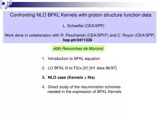
Confronting NLO BFKL Kernels with proton structure function data L. Schoeffel (CEA/SPP) Work done in collaboration with R. Peschanski (CEA/SPhT) and C. Royon (CEA/SPP) hep-ph/0411338 40th Rencontres de Moriond • Introduction to BFKL equation • LO BFKL fit to F2(x,Q²) [H1 data 96/97] • NLO case (Kernels + fits) • Direct study of the resummation schemes • needed in the expression of BFKL Kernels
Introduction to BFKL equation (in DIS) F2 well described by DGLAP fits What happens if S Ln(Q²/Q0²) << S Ln(1/x) ? => Needs a resummation of S Ln(1/x) to all orders (by keeping the full Q² dependence) => Relax the strong ordering of kT² => We need an integration over the full kT space xG(x,Q²) = dkT²/kT² f(x,kT²) * BFKL equation relates fn and fn-1 (fn = K fn-1) => f(x, kT²) ~ x- kT diffusion term => increase of F2(x,Q²) at low x… p
F2 expression from the BFKL Kernel at LO After a Mellin transform in x and Q², F2 can be written as F2(x,Q²) = dd /(2i)² (Q²/Q0²) x-F2(,) At LO F2(,) = H(,) / [ - LO()] with = S 3/ LO() is the BFKL Kernel ~ 1/ + 1/(1-) For example DGLAP at LO would give ()~1/ H(,) is a regular function and the pole contribution = LO() leads to a unique Mellin transform in . Then, a saddle point approx. at low x => F2(x,Q2) = N exp{½L+YLO(½)-½L2/(’’LO(½)Y)} ~ Q/Q0x-= (½) L = Ln(Q2/Q02) et Y = Ln(1/x) Note : c = ½ is the saddle point
Results at LO F2(x,Q2) = N exp{½L+YLO(½)-½L2/(’’LO(½)Y)} ~ Q/Q0x-= (½) L = Ln(Q2/Q02) et Y = Ln(1/x) Very good description of F2 at low x<0.01 with a 3 parameters fit // global QCD fit of H1… We get : Q0² = 0.40 +/- 0.01 GeV² and = 0.09 +/- 0.01 [ = S 3/] => Much lower than the typical value expected here ~ 0.25 => Higher orders (NLO) corr. needed with S running (RGE)… F2 (measured by H1 96-97 data)
BFKL Kernel(s) at NLO = LO case NLO BFKL Kernels (,,) Calculations at NLO => singularities => resummation required by consistency with the RGE (different schemes aviable) • Consistency condition at NLO • NLO(, , RGE) verifies the relation : • = p = RGE NLO(, p,RGE) // LO condition = LO() Numerically => p(,RGE) Then we get : NLO(, p,RGE) eff(,RGE)
Deriving F2(x,Q²) from BFKL at NLO Saddle point approximation in (// LO case) : F2(x,Q2) = N exp{cL+RGEYeff(c, RGE)-½L2/(RGE’’eff(c,RGE)Y)} L = Ln(Q2/Q02) et Y = Ln(1/x) with c =saddle such that ’eff(c,…) = 0 NLO and LO values of the intercept are compatible For a reasonnable value of RGE
Results at NLO F2 compared with LO predictions and 2 schemes at NLO… Sizeable differences are visible between the two resummation schemes at NLO The LO fit (with 3 param.) gives a much better description than NLO fit (2 param.) for Q²<8.5 GeV² => Pb with the saddle pt approx? => Pb with the NLO Kernels?
Study of the consistency relation at NLO Determination of saddle(,Q²) From F2(,Q²) = d/(2i) (Q²/Q0²)f(,) => ∂lnF2(,Q2)/∂lnQ2 = *(,Q2) Then we can determine *(,Q2)~saddle from parametrisations of F2 data(x,Q²) -> F2(,Q2) -> saddle Then, we will study the consistency relation = RGE(Q2) NLO(*(), ,RGE) (reminiscent from the similar relation at LO)
Consistency relation From *(, <Q2>) => we determine NLO(*,,RGE) • and verify the relation • NLO(*,,RGE)=/RGE(<Q2>) ? • In black : NLO(*,,Q²) • In Red : /RGE(<Q2>) • The consistency relation does not hold exactly BUT NLO(*,,Q²) is linear in and does not diverge => spurious singularities properly resummed! (it is not the case for all schemes…) In practice we have : NLO(*,,RGE) ~ / OUT Note : Recalculating eff with this relation does not change the results on the F2(x,Q²) fits…
Summary • Effective approximation of the BFKL Kernels at NLO • => 2 parameters formula for F2(x,Q²) at low x<0.01 => Reasonnable description of the F2 data => Sensitivity to the resum. schemes + pb with the 2 lowest Q² bins… • Direct studies of the resum. schemes in Mellin space => The consistency relation holds approximately => Discrimination of the different schemes / existence of spurious singularities Further studies : * Beyond the saddle point approximation : unknown aspects of prefactors could play a role (NLO impact factors…) * New resum. schemes…